Full-field Data Tools

The proliferation of full-field data acquisition systems and tools, such as digital image correlation (DIC) and infrared (IR) cameras, provides a plethora of data to be used for model calibration and validation activities. Generally, full-field data is more complicated to work with than conventional probe data, because of this it has conventionally only been used for qualitative comparisons. Full-field data sets are noticeably more difficult to work with than probe based data sets because of two main factors. The first factor is the additional dimensionality of the data, where conventional data only requires alignment in time(or some analogous measure), full-field data requires alignment in both space(typically two dimensional) and time. The second factor is the sizes of data involved in full-field calculations. Where conventional experimental measurements and simulation predictions only produce data sets with a few columns and many rows, full-field data sets produce data sets with many columns and many rows. This increase in data size takes what was a trivial memory requirement on modern computers, and makes it a significant concern. These two challenges make writing a full-field calibration code difficult, and with few appropriate external libraries to help.

Full-field data used in concert with probe measurements has the potential to provide much more insight in to the material behavior than with probe measurements alone. Potential benefits of using full-field data include:

Potential to reduce the number of experiments required to characterize data. Full-field data collection techniques extract more information per experiment, potentially allowing researchers to gain the necessary amount of information to characterize a material with less experiments.
Increased model form scrutiny. Probe measurements often provide an integrated, homogenized, or partial measurement of the changes happening during an experiment. Full-field data provides many local experimental observations that provide a fuller measurement of the material evolution during an experiment. This fuller picture can reveal weaknesses in a material model’s representation much more apparently than by probe measurements alone. This clarity allows the analyst to identify potential weakness in their model and can take steps to address them.
Enabling of fast ‘solver free’ calibration techniques. Full-field data often provides the degrees of freedom that are solved for in engineering software. This information allows for the use of techniques that avoid much of the necessary calculations done in these codes, allowing for calibrations to finish in a fraction of the time compared to conventional calibrations.

To leverage the benefits that full-field data can provide MatCal has three full-field data analysis methods:

Meshless Interpolation
Virtual Fields Method
Hierarchal Wavelet Decomposition

These methods range from common to novel and provide tools that quantitatively compare full-field data from two different sources which enables model calibration and validation. In addition to providing calibration methods for full-field data, MatCal includes tools for easier manipulation and of surface full-field data.

All of these tools can be used for the following tasks:

Material model calibration with MatCal calibration studies. See local_calibration_studies and global_calibration_studies.
Model validation by comparing model results to experimental using MatCal objectives. See InterpolatedFullFieldObjective, PolynomialHWDObjective and MechanicalVFMObjective.
Model parameter sensitivity and uncertainty quantification studies. See sensitivity_studies, uncertainty_quantification_studies and LaplaceStudy.

Warning

MatCal currently does not attempt to align full-field data from two different objects before operating on it. The user must ensure that the data are properly aligned in two-dimensional space before using MatCal’s tool for full-field mapping or comparisons.

Full-field Interpolation and Extrapolation

For full-field interpolation and extrapolation, we use the python implementation of the Compadre Toolkit [2, 15]. From the Compadre Toolkit, we use the generalized moving least squares method (GMLS) to interpolate and extrapolate from one point cloud to another. Usually, we are using this tool to map fields from the experiment data cloud to a computational discretization. This workflow was chosen as our default operation in order to conserve memory and decrease computational cost. The computational cost is reduced in terms of both cpu time and memory for the following reasons:

When we interpolate on the experimental data to the simulation discretization, we can store the mapped experimental data at the simulation discretization locations and compare directly to simulation output. As a result, we would only perform the mapping upon initialization and not every time the model is evaluated. The mapping process requires non-negligible computational cost in terms of cpu time and memory, so this reduces the overall computational cost for each evaluation.
For Digital Image Correlation (DIC), which measures full-field displacements over a domain, the experiment point cloud is frequently denser than the simulation discretization. During a calibration, if we had to interpolate from a coarser discretization to a finer one, we would be up-sampling the data and increasing our memory foot print for each simulation result evaluated without affecting the results for a given simulation discretization. In calibrations problems, this additional memory expense can become significant if many models and time steps are needed for every objective function evaluation.

Generalized Moving Least Squares Theory

A basic overview of the Compadre GMLS theory is presented here. For our purposes of data interpolation and extrapolation, we use the Compadre GMLS solver to solve a traditional moving least squares problem. As a result, we will describe the theory for the moving least square problem. For more details see [33]. Moving least squares solves a local, weighted least squares problem to approximately reproduce a function $f\left(x\right)$ from a discrete set of values for $f$ known at locations $X = \left\{x_1, ..., x_n\right\}$ . The approximation of $f$ , $f^h$ , is determined by the solution of

(11) $\min\left\{\sum\left[f\left(x_i\right)-p\left(x_i\right)\right]w\left(x,x_i\right)\right\}$

where $p$ is a polynomial of a pre-specified order, and $w$ is a weighting function specific to the current point of interest $x_i$ .

In order to reduce the cost of the least squares, the weights for the least squares problem are designed so that only points within some distance away from the point of interest are included making it a local least squares problem. This is done using a weight function with local compact support such that it is one near the point of interest and drops to zero some distance away from the point of interest. The weighting function used by the python interface to Compadre is a power weighting function of the form

(12) $w\left(r,n,p,h\right) = \left(1-\left|\frac{r}{h}\right|^n\right)^p$

where $n$ and $p$ are parameters governing the weighting function shape, $h$ is the radius of compact support for the function and $r$ is the Euclidean distance from the current point of interest. By default, the weighting function exponents are set such that $p=2$ and $n=1$ . By setting up the least squares problem in this way, the system to be solved is sparse and the fitted function can be calculated using efficient methods.

After solving the minimization problem defined in (11), we have an analytical function, $f^h$ , that can be used to estimate the value of $f$ at any point $x$ . Note that $x$ should be within or close to the domain of the function space where $f$ is measured $x_i$ to avoid extrapolating.

Warning

MatCal will use $f^h$ to extrapolate. This is necessary to support VFM calibrations using DIC data that is not defined near the test specimen edged. Care must be taken to ensure the extrapolation values are valid. We choose parameters for the GMLS algorithm in an effort to make the method robust and reliable, however, these parameters may need to be changed depending on the your data and modeling choices. See Full-field Interpolation Verification for more information on how these parameters were chosen.

MatCal’s GMLS Implementation

MatCal interpolates using Compadre’s python implementation pycompadre. Compadre leverages the advantages of the Kokkos library to perform the calculations necessary for GMLS in a scalable parallel fashion. MatCal wraps the various tools used by pycompadre, so that there is a limited need to understand the implementation details of Compadre by the rest of the code. The main tools of interest that use GMLS are the function meshless_remapping() and InterpolatedFullFieldObjective.

The meshless_remapping() function is used throughout MatCal to perform the unstructured interpolation from one point cloud to another point cloud. This function is also available with the default import of MatCal, providing users easy access to the ability to interpolate between two unstructured point clouds. The function stores no information between calls, therefore it is best to submit as much information in one large batch call as possible. Large batch calls avoid the need for the recreation of the interpolation weights which occurs each time the function is called. For more details on how to use meshless_remapping() please see the function’s API documentation.

The InterpolatedFullFieldObjective is the way that MatCal generates an objective based on interpolating an experimental point cloud data to node locations from a simulation. MatCal expects nodes from a single surface of a simulation, but does not require any connectivity information about the surface. Therefore simulation results from finite element like simulations and meshless simulations can both be calibrated. the InterpolatedFullFieldObjective uses the same underlying wrapping tools that meshless_remapping() uses. In this objective the experimental full-field data is interpolated onto the simulation nodes in space and the simulation values are interpolated in time to the experimental time stamps (Table 1).

Table 1 Interpolation Direction
	Space	Time
Experiment	From	To
Simulation	To	From

These directions were chosen because they interpolate from the more dense data set to the less dense data set. Full-field experimental data points are often much more dense than the computational nodes, and experimental data sets can often efficiently be down-sampled in time without losing important information to be less dense than computational time step requirements. Interpolating this way minimized the data requirements per evaluation, and helps ensure that there is enough computational support to meaningfully interpolate.

In addition to the point cloud data supplied to these tools, the key values that the user needs to supply to the methods is the order of polynomial to use and the search radius multiplier. The first one is the polynomial order used to approximate the field and the other effectively changes the number of reference points used in the local polynomial fit. More details about these terms can be found in section Full-field Methods Verification.

MatCal uses GMLS for extrapolation in space. MatCal does not separate its interpolation and extrapolation workflows. Keeping the two together means that they share the same polynomial order and search radius. Extrapolation often performs best with lower polynomial orders, while interpolation performs better with higher. MatCal has a default of polynomial order of 1 and search radius multiplier of 2.75, as these values seem to perform reasonably well in both extrapolation and interpolation for data sets we have seen.

Virtual Fields Method

The Virtual Fields Method (VFM) uses the principle of virtual work to balance the internal virtual work within a specimen with the external virtual work on the same specimen for material model calibration. When combined with full-field data measurement techniques, such as digital image correlation, we can use the measured displacement field to determine the material stress state under a plane stress assumption which allows for rapid model evaluation and efficient material model parameter identification [22].

While the formulation of VFM is agnostic to the application, in practice it is difficult to apply it out side of solid mechanics. This is because it is difficult to accurately represent the boundary conditions well enough to use in many other physics.

VFM Theory Overview

For the case of finite deformation where inertial and body forces are ignored, the principle of virtual power is used

(13) $\int_{V_0} \mathbf{\Pi} : \dot{\mathbf{F}}^*dV = \int_{\partial V_0} \left(\mathbf{\Pi} \cdot \mathbf{n}_0 \right) \cdot \mathbf{v}^* dS$

where $V_0$ is the body in the reference configuration, $\Pi$ is the first Piola-Kirchhoff stress, $\dot{\mathbf{F}}^* = \frac{\partial \mathbf{v}^*}{\partial \mathbf{X}}$ , $\mathbf{v}^*$ are the virtual velocity fields, and $n_0$ is the surface normal in the reference configuration [25]. The surface traction on the boundary in the external power term cannot be easily measured, however, the total force on the surface is easily measured with a load cell. In order to simplify the external power term, a virtual velocity function is chosen such that the function is constant along the boundary of loading. As a result, the virtual power balance simplifies to

(14) $\int_{V_0} \mathbf{\Pi} : \dot{\mathbf{F}}^*dV = \mathbf{f} \cdot \mathbf{v}^*$

where $\mathbf{f}$ is the measured external load along the boundary. If desired, the virtual power can be integrated to obtain the virtual work. For our purposes, we will work with the virtual power to allow more flexibility within MatCal’s optimization framework.

With the virtual power balance, a residual can be formed where inputs are the external load on the test specimen, a set of kinematically admissible virtual velocity functions, and the first Piola-Kirchhoff stress at any point in the body. To calculate the first Piola-Kirchhoff stresses in the body, the measured displacement field is mapped to a finite element mesh. Adopting a plane stress assumption, this mesh is used to determine the plane stress kinematics for the supplied displacement field and provide the appropriate strain measures needed to determine the stress state in each element. Given a set of material parameters, a material point solver can then be used to return the correct stresses from the calculated kinematics. Then the internal power integral can be calculated easily on the finite element mesh.

In a practical application, full-field data is represented as several discrete points in time, these timestamps then define the individual points where an individual residual is calculated. Lastly, a total objective is calculated using an objective metric to combine the virtual work residuals over the time frame of interest or the residual for each time step can be used in a nonlinear least squares solver.

In summary, the VFM method reformulates the calibration problem, such that it takes in experimental DIC data, boundary loading data, and a set of parameters to directly produce a residual, and skip the conventional finite element solve required for most other calibration methods.

For a given set of experimental data, producing a mesh of the specimen of interest can be accomplished with traditional meshing software. The virtual velocity functions can be any kinematically admissible function which means they must be constant at the loading boundary so that the simplified virtual power equation in (14) is valid. As a result, they are easily defined. Difficulties in using VFM arise in few places:

Data manipulation and importing.
Mapping the data to an appropriate finite element mesh.
Solving the element kinematics and material model.
Interfacing with an optimization routine.

Each of these steps require specialized software tools to make the process efficient and with an approachable user interface. MatCal aims to address these issues in our production VFM capability.

MatCal’s VFM Implementation

Note

The thickness direction is the Z direction and the loading direction must be the Y direction. User provided meshes and data should conform to these directions.

Warning

SIERRA/SM is inherently 3D and, as implemented, the VFM models may produce non-negligible through the thickness stresses depending on the boundary value problem being simulated. In the virtual internal work calculation, all through thickness stresses are currently ignored. This leads to errors in calibration, however, if the boundary value problem conforms well to the plane stress assumption these errors should only be on the order of 1% or less for the parameter values.

Warning

The experimental full-field data must be properly aligned with the mesh. We currently do not assist in aligning the mesh coordinate system with the experimental data coordinate system. Work with the experimentalist to do so or perform alignment as a preprocessing step.

MatCal’s VFM implementation provides the software tools needed to simplify using VFM for engineering applications. This work was inspired by previous research efforts at Sandia related to VFM [10, 14]. These efforts highlighted potential benefits for using VFM for material parameter identification, but did not result in tools that the general analyst could use in production setting. Building off these previous works, we implemented VFM tools that could be easily distributed, easily modified and used for research and applied engineering problems. Specifically, we address the issues discussed at the end of Virtual Fields Method, addressing data importing (see Full-field Data Specific Features), full-field data mapping, the finite element kinematics, material modeling and interfacing with an optimization algorithm. We do this through the development of our own tools and relying on several external libraries and codes. The tools we have available and their limitations are discussed or linked to in this section.

Full-field Data Mapping for VFM Models

We currently use MatCal’s interface to PyCompadre for GMLS based data mapping for full-field data interpolation and extrapolation. The mapping is performed automatically for the user. However, the user must ensure that the point cloud data being used as the boundary condition data in the VFM model is appropriately aligned with the mesh they are using for their VFM model. With a properly aligned point cloud and mesh, the VFM model will map the in-plane displacements and, if necessary, full-field temperatures onto the VFM model mesh.

See Full-field Interpolation and Extrapolation and Full-field Interpolation Verification for more details on the GMLS interpolation methods.

Element Kinematics and Material Modeling

MatCal currently does not support any element kinematics calculations or material model solvers. We rely solely on Sierra to perform these functions for us. However, due to restrictions on available interfaces to Sierra algorithms, we do so all through a full Sierra finite element (FE) model that is solved using implicit quasi-statics for the field data provided. We currently have two VFM models available for users. Both use hexahedral elements and are a single element thick with all in-plane displacements prescribed from the provided full-field data that is mapped to the mesh nodes. These models are valid for thin sheet problems exhibiting plane stress for which VFM was originally derived. Since SierraSM does not fully support plane stress elements, some through-the-thickness nodal degrees of freedom must still be solved for in the model. Although a full FE simulation is still performed, the significantly reduced degrees of freedom due to the fully prescribed in-plane boundary conditions and reduced density of the stiffness matrix reduces the computational cost of the model solve considerably.

The largest benefit of VFM is that it the FEA solver is now solving a series of independent material model instead of one large coupled FE model solve. Even though our implementation does not fully realize this, we do realize several other benefits that out weigh this single draw back.

We are able to access all SierraSM material models and all the testing, verification and validation that comes along with them. Otherwise, users or developers would have to make their own versions compatible with python and our classes and interfaces. This task is nontrivial.
We can benefit from all FE model functionality that may be of interest to users and is included in Sierra. Most importantly from these features, we support adiabatic heating with material model temperature dependence. For one of the two VFM models provided by MatCal, we can solve heating due to plastic work and any conduction that may occur throughout the body.
We get some computational cost benefit from any speed related feature that is built into SierraSM. These include parallelism, any speed improvements implemented in the material models themselves and the eventual adoption of GPUs.

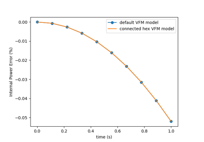
As alluded to previously, we have two VFM models available for MatCal studies. Both are valid for only uniaxial loading and use hexahedral meshes. The VFMUniaxialTensionHexModel is the recommended model to use for most cases. It has the advantages of being the least computationally expensive and most robust of the two models. Its single disadvantage is that it cannot model heat conduction. For intermediate loading rates where heating and conduction is expected temperatures must be measured during the experiments. For cases where heating due to plastic work and conduction are important, the VFMUniaxialTensionConnectedHexModel is available, but will be more computationally expensive and potentially less reliable. This model has the advantage of being able to solve the conduction problem with the disadvantages of less robustness and increased cost. Another advantage is better representation of out-of-plane deformation due to the continuity enforcement across elements and the the use of a through-the-thickness symmetry boundary condition on one of the out-of-plane surfaces. As a result, this model effectively has two elements through the thickness of the thin specimen being simulated.

For more information about these models and their specific features, see Virtual Fields Method Uniaxial Tension Models.

Warning

Several reminders of constraints and potential issues for the VFM models are included here once again:

The out-of-plane stresses are currently ignored. However, we have plans to include them in future releases an effort to attempt using VFM past peak load for specimens that plastically localize and exhibit non-negligible out-of-plane stresses.
Currently, the VFM models can only be used to simulate test specimens with loading along a single axis.
Careful mesh alignment with the source field data for displacement data is critical to obtain correct results.

VFM Interfacing to MatCal Studies

Using MatCal’s VFM models in MatCal studies such as calibration studies or uncertainty quantification studies requires only the use of one of the MatCal’s VFM models, the creation of a MechanicalVFMObjective object, and global load-time data for the external virtual work calculation.

The MechanicalVFMObjective performs the calculation of the virtual power residuals. It has two optional input parameters of the field names in the supplied experimental data for time and external global load. By default, it assumes the fields are named “time” and “load”, respectively, for these two data fields, but the user can change the names if needed. We currently only support the virtual velocity functions that were presented in [10]. They take the form

(15) $\mathbf{v}^*_X=\cos\frac{\pi\bar{Y}}{h}$

(16) $\mathbf{v}^*_Y=\frac{2\bar{Y}+h}{2h}$

where $Y$ is the direction of loading, $\bar{Y}$ is the centered position of the current point of interest in the reference configuration, and $h$ is the total height of the data. The data points $Y$ are centered using

(17) $\bar{Y}=Y-\left(\frac{h}{2}+\min\left(\mathbf{Y}\right)\right)$

where $\mathbf{Y}$ is a vector of all the Y direction coordinates from the points of interest. As implemented in MatCal, $\mathbf{Y}$ is used from the VFM model not the experimental data since the experimental data may not extend fully to the edges of the gauge section. Research has shown that the virtual velocity functions can be chosen to improve objective sensitivity to the input parameters [18, 19, 20]. These techniques have yet to be implemented in MatCal but could be implemented in future releases.

After creating a VFM model and a MechanicalVFMObjective, any available MatCal study can be performed using them by adding them to the study with add_evaluation_set(). Since the model is the only component in the evaluation set that requires full-field data, this method takes data in the form of matcal.core.data.Data, matcal.full_field.data.FieldData or matcal.core.data.DataCollection objects. The study will then compare the internal virtual power from the model to the external virtual power from all applicable experiments to form a residual for the evaluation set. If desired, additional evaluation sets can be added to the study with any supported MatCal model and data type. This would result in a hybrid VFM model and traditional FE model study and may be required if full-field data could not be taken for all material characterization tests or the plane stress assumption does not apply to some of the characterization tests.

VFM next steps

With the base features in place, extensions and additions can be explored as future work. Potential features and research activities include:

A general VFMPythonModel will fully realize the primary benefit of VFM and is of use to organizations and groups that do not use Sierra. We will provide a few standard material models and a interface for users to implement their own.
Inclusion of out-of-plane stresses into the internal virtual work calculation.
Optional addition of extra element layers in the VFMUniaxialTensionConnectedHexModel().
General extension of the VFM models and tools to three-dimensions.
Implementation of sensitivity-based virtual velocity functions.

Hierarchical Wavelet Decomposition

Hierarchical Wavelet Decomposition (HWD) attempts to represent large unstructured data as a series of pattens. Representing the data as patterns allows for compression of the residual size required to analyze the data, allowing larger problems to be run, and potentially allowing for more meaningful interpretations of the data than could be observed though direct observation of the unstructured data set. In MatCal HWD is primarily used to create a latent space on which full-field data is compressed. Compressed full-field data allows HWD based parameter studies to use full-field data in the same way as an interpolated based objective, however at a much lower memory footprint.

HWD Theory

HWD at its core is a linear projection of a data set onto a series of orthogonal bases that characterize the data seen in the data set. There are many forms of projection based methods, with Principal Component Analysis (PCA) being one of the most common methods uses. In equation (18) shows the general setup for this type of method.

(18) $\underline{d} = \underline{\underline{Q}} \cdot \underline{c}$

Where $\underline{d}$ is the unstructured full-field data, $\underline{\underline{Q}}$ is the matrix of bases vectors, and $\underline{c}$ are the weights of the bases vectors used to recreate the original field data. The data vector $\underline{d}$ is of length $n$ . This means that the bases matrix $\underline{\underline{Q}}$ is of shape $n \times m$ where $m$ is the number of bases vectors. It is desired that $n >> m$ , such that the compressed weights are much smaller than the initial data set, but effectively contain as much information as the initial data set.

It is common to define $\underline{\underline{Q}}$ to be orthogonal. Which means that all bases vectors in $\underline{\underline{Q}}$ contain unique information. Orthogonality also, allows for a simple inversion of $\underline{\underline{Q}}$ , buy taking its transpose, and therefore allowing one to find the values for the weights by using equation (19).

(19) $\underline{\underline{Q}}^T \underline{d} = \underline{c}$

The challenge is projection based methods is identifying an appropriate set of bases on to which to project the data. Often the approach taken is to generate a sufficient about of data and directly build a bases based off a corpus of pre-computed results. While this method generates great compression ratios for a given data set, it has a large upfront cost that can be intensive to generate. This means that for initial exploratory parameter studies methods that rely on a pre-computed corpus of data, like PCA, can be prohibitively expensive. HWD attempts to provide a similar service to PCA, but without the requirement for a pre-computed corpus of data.

HWD combines the approaches of Salloum [26] and Christian [23]. To generate a series of orthogonal wavelets at various length scales across the data. The core steps to generate the basis matrix using HWD consists of 3 steps:

Generation of hierarchical tree to represent of the physical space occupied by the full-field data
Generation of approximation functions at the various levels of the tree
Use of QR Decomposition to generate an orthogonal basis( $\underline{\underline{Q}}$ .) and a change of basis matrix( $\underline{\underline{R}}$ .)

Additional steps, or sub-steps my be required to properly process the data or generate a more informed bases, but at its core these are the main steps used in HWD. HWD builds upon [26] and [23], by taking the QR factorization approach of [23] and applying it to a hierarchical split domain from [26].

As identified by [23], applying patterns directly to different unstructured data sets generates compressed forms that are similar, but are not the same. While similar but not the same may be sufficient for some applications, for the its use in applications like material calibration such a discrepancy is not useful. Their solution was to build their basis from an initial background series of polynomials. These polynomials are defined in space covering the domain of the data points, but not bound to the points themselves. these polynomials are evaluated across all points in a given data set to generate a moment matrix $\underline{\underline{M}}$ . Each column of the moment matrix is the evaluation of one polynomial in the series, with the rows being the evaluation result for a given point. The moment matrix is then decomposed in to an orthogonal basis( $\underline{\underline{Q}}$ .) and a change of basis matrix( $\underline{\underline{R}}$ .) via QR factorization.

The factorization of the moment matrix provides the $\underline{\underline{Q}}$ necessary to generate weights using (19), but also supplies a method to map the weights from one data set to an other. In equation (20), the change of basis matrices are used to map the weights from data set 1 to be compatible with data set 2. The mapped weights now can be compared much more rigorously.

(20) $\underline{c}_{12}= \underline{\underline{R}}_2 \underline{\underline{R}}_1^{-1} \underline{c}_1$

Using equation (20) a calibration residual can be defined by labeling one of the data sets as the reference(or experimental) and subtracting it by the mapped weighted simulation data, like in equation (21).

(21) $\underline{r}= c_{ref} - \underline{\underline{R}}_{ref} \underline{\underline{R}}_{sim}^{-1} \underline{c}_{sim}$

HWD extends the work of [23] by generating an initial moment matrix that takes into account both large scale and small scale patterns that may be present in the data. HWD does this by using a binary tree to successively split the physical space of the data, and then applying pattern functions(typically polynomials) to all the regions generated by the tree splitting. Generating the splits for each section of the domain can be done in a variety of ways, but is usually done by using clustering algorithms to split regions into regions of greatest likeness.

Pattern functions are the functional forms chosen to populate the momentum matrix. Currently, polynomials are the only functions that have been extensively used, but other functional forms are valid choices as well. Future research is planned to investigate the optimal choice of functional form used for the pattern functions if some data is available.

By applying the pattern functions at different levels of spatial scale it is believed that important localized behavior should be captured better than if exclusively larger scale functions are used. In practice only one of the two regions generated by each split in the tree, has the pattern function applied to it. This is to preserve linear independence between the size scales, required to obtain the desired QR factorization.

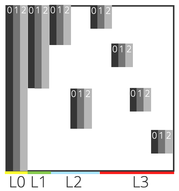
Example momentum matrix generated using a quadratic polynomial on one dimensional data. — Fig. 15 This is an example illustration of a momentum matrix generated by HWD. The data in this example is ordered one dimensional data, and the pattern functions chosen are polynomials up to order 2. The domain has gone though 3 layers of splitting. The colored regions at the bottom indicate the different tiers of splitting, while the numbers at the top indicate the order of polynomial used in that column.

After the tiered momentum matrix is generated, it is run though the same flow as [23]; a QR factorization is applied to the momentum matrix and a basis matrix( $\underline{\underline{Q}}$ ) and change of basis matrix( $\underline{\underline{R}}$ ) are formed. Then equations (20) and (21) can be used to define a residual, the only additional complication is that all data sets that want to be compared need to use the same splitting/clustering instance. By using the same instance, it will ensure that the different data sets are partitioned in the same way and have compatible bases.

MatCal HWD Implementation

MatCal implements HWD using polynomials through an external HWD library. The library can be found on the Sandia SRN at https://cee-gitlab.sandia.gov/mwkury/hierarchical-wavelet-decomposition. MatCal currently uses a reduced polynomial pattern function to generate its moment matrix in the HWD library. Because full-field data is two dimensional in space, generating polynomials of arbitrary order can generate an excessive amount of possible bases, without adding too much additional value. The reduced polynomial pattern function cuts down on the number of polynomial terms generated by only keeping the isolated X and Y terms (e.g. $X^3$ or $Y^2$ ) and only generating the middle cross term for a even polynomial powers (e.g. if the power is 4, then $X^4$ , $Y^4$ , and $X^2 Y^2$ will be generated). This helps preserve the effects that cross both X and Y, while keeping the number of bases from exploding out of control.

During the definition of an HWD objective, the user can supply the max polynomial order and the max sets of splits. Higher numbers of splits will also balloon the number of bases generated, and users are advised not to go above 8.

Due to the current naive implementation of the domain decomposition in the HWD library, the library does not make ideal choices when supplied point cloud geometries of complex shapes(such as those containing holes). Due to poor decomposition behavior, the the cross data set mapping is too poor to be used for material calibration. While the HWD library will be improved to create better domain splitting choices, a stop gap measure leveraging the generalized moving least squares (GMLS) algorithm tools in MatCal and pycompadre [15] is used to interpolate the experimental data sets on to the simulation data sets.

Performing the interpolation in the beginning, allows the remapping step (equation (20)) to be skipped, and the calculated weights to be compared directly, equation (22).

(22) $\underline{r}= c_{ref} - \underline{c}_{sim}$

In addition to the streamlined residual, performing an initial interpolation on to the simulation data points allows for an easy down-selection of bases vectors. Because the remap step potentially ties all weights together, removing that step allows us to ignore weights for bases that do not play an important role in describing data. MatCal supplies a tolerance ratio to the HWD library that governs the minimum magnitude of a basis weight required to be considered significant. Based on the first set of data supplied to the HWD library, the largest weight is identified and all bases with weights of lower magnitude than the tolerance ratio times the largest weight magnitude are discarded and only the remaining bases vectors and weights are used. This allows for additional compression of the residual, which is important because it allows for larger models to be used in parameter studies.

Full-field Methods Verification

In this set of examples, we perform verification exercises for MatCal’s full-field data methods. These examples provide verification of some of the tools that contribute to full-field data calibration. These verification examples are extensions to some of the tests that are required to pass for each MatCal update.

Full-field Interpolation Verification

Polynomial HWD Verification - Analytical Function

Polynomial HWD Verification - X Specimen Data

Polynomial HWD Verification with Colocated Points

Virtual Fields Method Verification

Gallery generated by Sphinx-Gallery

Full-field Study Verification

In this set of examples, we perform verification of MatCal studies using full-field data tools and objectives. There are several examples studies included here. We provide these examples in order to show the current best practices when calibrating to full-field data for solid mechanics problems and to highlight what benefits it can provide. We also highlight some challenges that may occur when using full-field data. Once successful calibration results are obtained, we compare the calibration results and the overall computational performance of the methods.

Full-field Verification Problem Material Model

For this example set, we model a non-standard specimen subject to uniaxial loading to generate synthetic data for the calibration. Our goal is to calibrate to these data and reproduce the parameters used to generate the data. In this section we will describe the model that we used to generate the synthetic data. First we describe the material model and geometry. We finish with a description of the generated data that will be used for calibration.

For the model we use a plastic material model with the Hill48 orthotropic yield surface [8] and Voce hardening [32]. We define the material flow rule using Voce hardening as

(23) $\theta^2\left(\boldsymbol{\sigma}\right) - \left[Y+A\left(1-\exp\left(-n\epsilon_p\right)\right)\right] \le 0$

where $Y$ , $A$ and $n$ are calibration parameters, and $\epsilon_p$ is the equivalent plastic strain of the material point. We use the Hill48 yield surface as our equivalent stress $\theta^2\left(\boldsymbol{\sigma}\right)$ where $\boldsymbol{\sigma}$ is the material Cauchy stress. The Hill48 yield surface is defined by

(24) $\theta^2\left(\boldsymbol{\hat{\sigma}}\right) = F\left(\hat{\sigma}_{22}-\hat{\sigma}_{33}\right)^2+ G\left(\hat{\sigma}_{33}-\hat{\sigma}_{11}\right)^2+ H\left(\hat{\sigma}_{11}-\hat{\sigma}_{22}\right)^2+ 2L\hat{\sigma}_{23}^2+ 2M\hat{\sigma}_{31}^2+ 2N\hat{\sigma}_{12}^2$

where $\boldsymbol{\hat{\sigma}}$ is the Cauchy stress rotated to a local material coordinate system and $F$ , $G$ , $H$ $L$ , $M$ , and $N$ are calibration parameters. These Hill48 parameters are typically not calibrated since they can be calculated using the yield stresses of the material in the six directions relative to the material directions. As a result, ratios for the material yield in each direction relative to some reference stress value are typically used for calibration. The ratios are defined by

(25) $R_{ii} = \frac{\sigma^y_{ii}}{\sigma_{ref}}$

and

(26) $R_{ij} = \sqrt(3)\frac{\tau^y_{ij}}{\sigma_{ref}}$

where $\sigma^y_{ii}$ and $\tau^y_{ij}$ are the material’s normal and shear stresses aligned with the material’s orthotropic material directions, and $\sigma_{ref}$ is an arbitrary reference stress.

We populate the material model with parameters that are representative of an austenitic stainless steel rolled sheet. The chosen parameter values are listed in Table 2.

Table 2 Chosen Material Parameters
Parameter	Symbol	Value
Elastic Modulus (GPa)	$E$	200
Poisson’s Ratio	$\nu$	0.27
Yield Stress (MPa)	$Y$	200
Voce Saturation Stress (MPa)	$A$	1500
Voce Exponent	$n$	2
$\sigma^y_{11}$ Ratio	$R_{11}$	0.95
$\sigma^y_{22}$ Ratio	$R_{22}$	1.00
$\sigma^y_{33}$ Ratio	$R_{33}$	0.9
$\tau^y_{12}$ Ratio	$R_{12}$	0.85
$\tau^y_{23}$ Ratio	$R_{23}$	1.0
$\tau^y_{31}$ Ratio	$R_{31}$	1.0

The synthetic material exhibits significant hardening, low yield and relatively mild anisotropy in yield. The anisotropy was added since it is a large driver for adding full-field data tools for calibration and validation activities. This is due to the fact that anisotropy can have a large effect on the deformation modes on deformed part while having less of an effect on the global load-displacement behavior.

Full-field Verification Problem Geometry

The geometry for this set of examples was chosen in an effort to require full-field data tools for an adequate calibration. The test geometry consists of a sheet with large notches and holes specifically placed such that depending on how the geometry is loaded the location of plastic localization changes. The thin sheet design was chosen to allow VFM to be used which requires a plane stress assumption.

The change in plastic localization location is driven by both the material model and the geometry. To achieve this, the two possible failure locations were designed to have similar lengths. These are shown in Fig. 16.

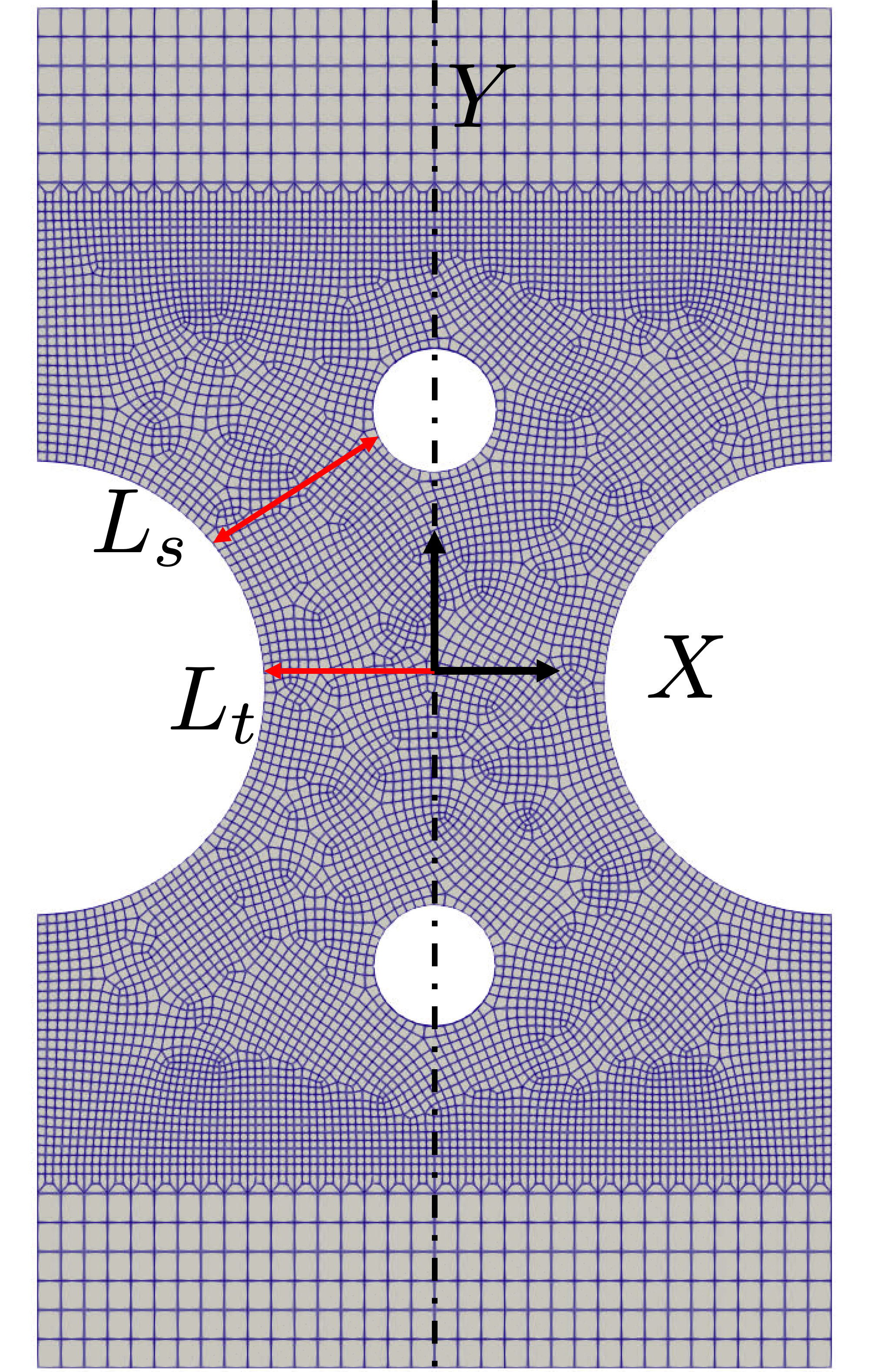
_images/study_verification_example_geometry.png — Fig. 16 The geometry used for the full-field data study verification examples. The specimen is loaded along the vertical axis shown with the dashed black line.

The two dimensions $L_s$ and $L_t$ are set so that they are approximately equal. The stress state in the region of $L_s$ is intended to be shear dominated while the region near $L_t$ is primarily loaded in tension. In Fig. 16, the material directions align with the global coordinate system shown. The material 22 direction aligns with the Y axis and the material 11 direction aligns with the X axis. This will be referred to as the 0_degree state. We also simulate another configuration that will be referred to as the 90_degree state. In the 90_degree state configuration, the material 11 direction is aligned with the Y axis and the material 22 direction is aligned with the X axis. Full-field data is only output from the more finely meshed region of the specimen and only on the largest in plane surface. This surface would be similar to what would have measurements from a test with digital image correlation measurements.

Full-field Verification Problem Modeling Information

There are a few details worth noting about the model used to generate the synthetic data.

The model is stopped once the load has dropped 50% from peak load. This is to save on simulation time.
Output is only requested on the region of interest to keep memory usage low. This can be done using SierraSM’s newer output features. Use output mesh = exposed surface and include = {surface_name} in your SierraSM Exodus output block to get output only on a side set named “{surface_name}”.
Tight residual tolerances and many time steps are used in an attempt to ensure finite difference derivatives of the calibration objectives with respect to the material parameters are accurate.
Since this is a verification problem designed to be computationally inexpensive, a mesh convergence study was not performed. A converged mesh is not required as long as the calibration mesh matches the mesh used to generate the synthetic data.
Symmetry was used on the Z plane. Due to mesh asymmetry, the results across the X plane were not symmetric which is believed to be more representative of experimental data. Although we could have enforced symmetry along the X plane, we did not.

The first three points are important to note and should be considered for all calibrations. The last two points are specific to our verification testing here.

Full-field Verification Problem Results

As stated previously, the problem was designed such that loading it in different directions produce different regions of plastic localization. This is accomplished through the similar lengths of $L_s$ and $L_t$ and the in-plane Hill48 yield ratios $R_{11}$ , $R_{22}$ , $R_{12}$ . If this were modeled using a von Mises yield surface, the part would always localize and fail in the center along $L_t$ . The stress in the component is shown at peak load for both the 0_degree and 90_degree states in Fig. 17.

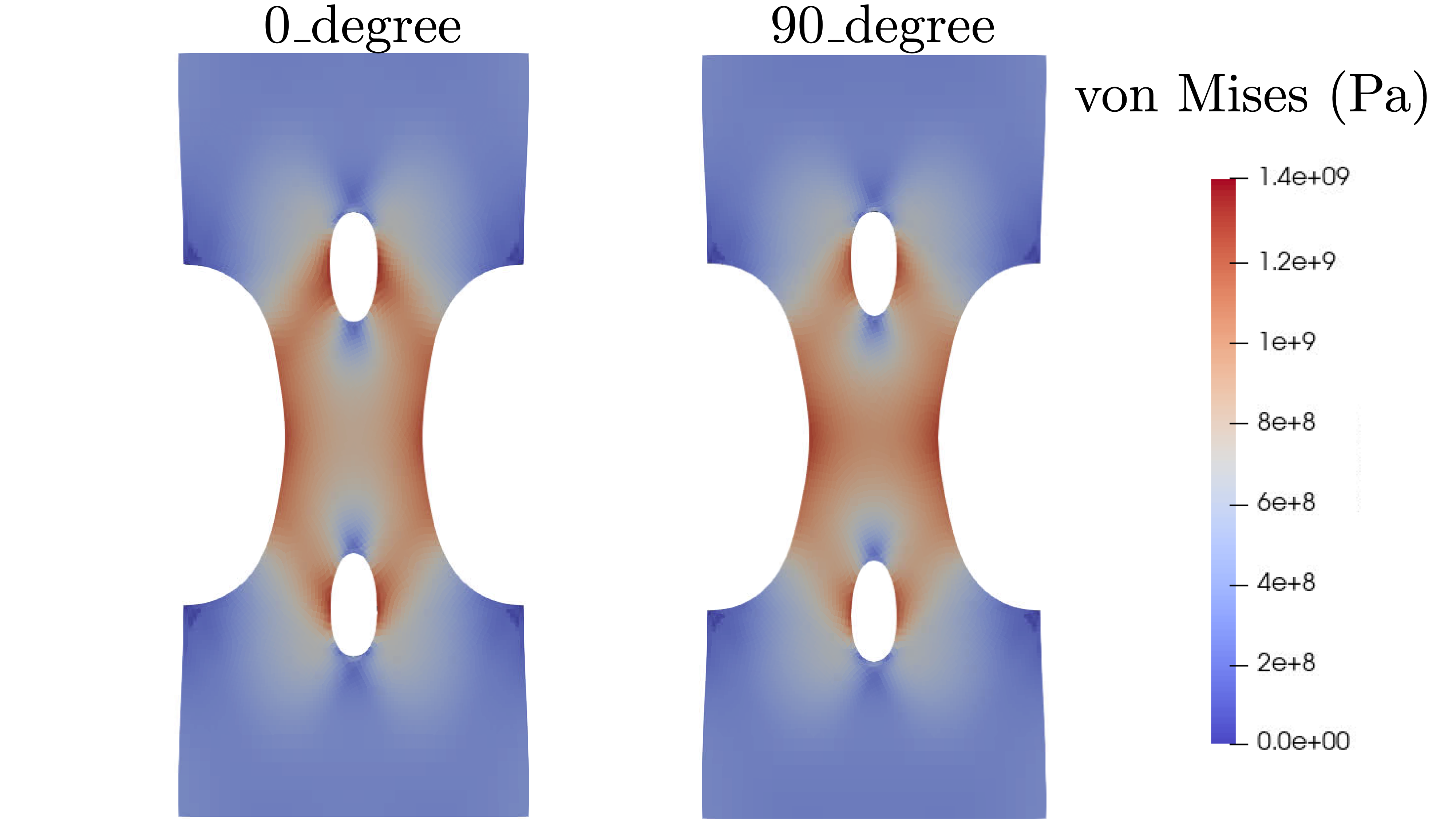
_images/study_verification_example_stress_peak.png — Fig. 17 The von Mises stress at peak load for each state. The left is the `0_degree` state and the right is the `90_degree` state.

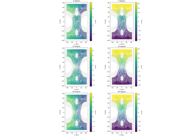
The stress fields look fairly similar with only a slight bias toward the $L_s$ region for the 0_degree and the $L_t$ region for the 90_degree. The localization is clear when looking at the plastic strains in the model after peak load as shown in Fig. 18.

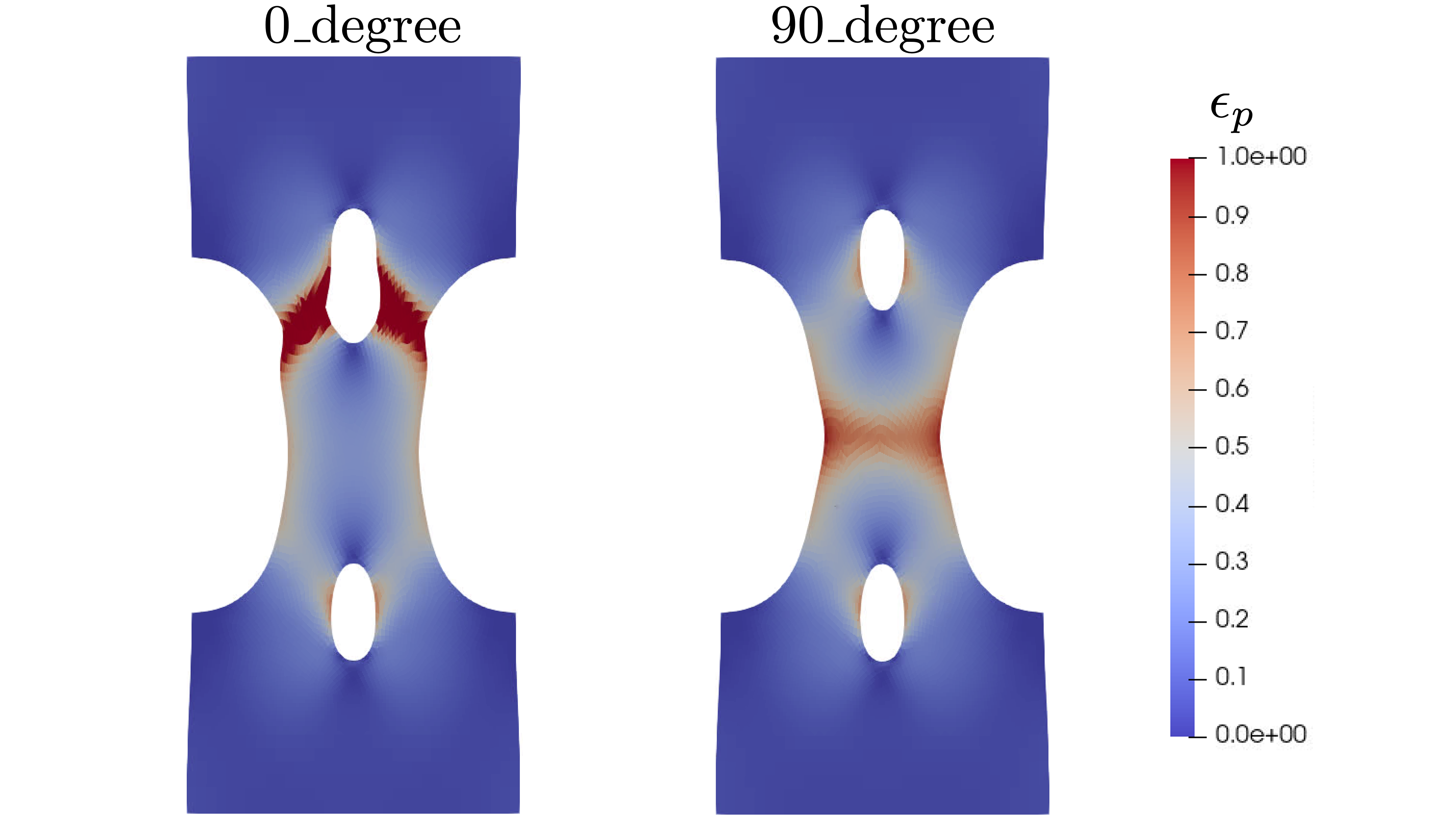
_images/study_verification_example_localization.png — Fig. 18 The equivalent plastic strain is shown at the end of the simulation (10 seconds) for each model. The left is the `0_degree` state and the right is the `90_degree` state.

The load-displacement curves also exhibit noticeably different behavior. They are shown in Fig. 19. for both simulated configurations. As expected, the specimen loaded in the material 22 direction has higher load carrying capacity due to the larger $R_{22}$ value. Due to the different localization regions, the load displacement curves unload at different rates.

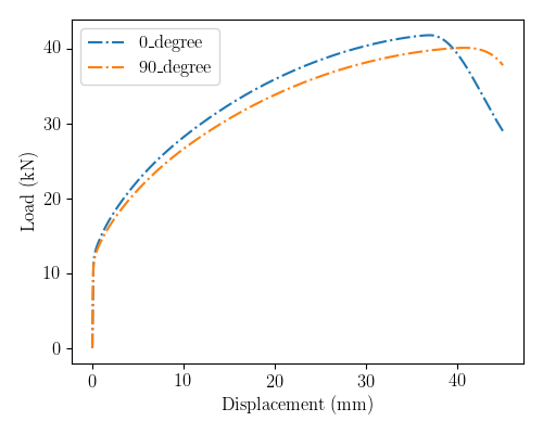
_images/study_verification_example_load_displacement.png — Fig. 19 The generated load displacement curves are shown here for each simulation.

Full-field Verification Study Examples

In this section, we present many studies in an attempt to perform the calibration. The ultimate goal is to use one state, either the 0_degree state or 90_degree state, to perform the calibration an obtain calibrated parameters within a few percent of the input parameters presented in Table 2. In practice, this is more difficult than it seems. The calibration focuses on only five of the eleven total material parameters. We only calibrate $Y$ , $A$ , $n$ , $R_{11}$ and $R_{12}$ . We assume that elastic parameters can be found in the literature and that only the in plane Hill48 ratios can be calibrated with the sheet-like specimen. We also set our $\sigma_{ref} = \sigma^2_{22}$ which requires that $R_{22}=1$ which is a common practice.

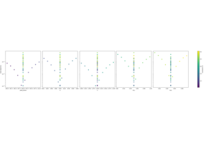
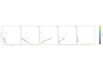
With the five calibration parameters chosen, we first verify that the objectives are all sensitive to these parameters. We perform a MatCal ParameterStudy where each parameter was changed -5% to +5% from its initial value and the full-field objectives in MatCal were evaluated for each parameter set. This was done to investigate shape of the objective function near the preselected parameter values used for the synthetic data generation. 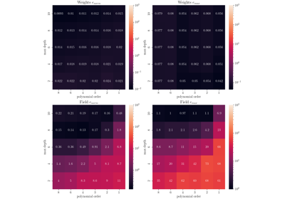Ideally, the objective will be lowest at the values specified in Table 2 and smoothly increase away from them. As can be seen in Objective Sensitivity Study, the objectives are all sensitive to the input parameters and return the lowest objective at, or in the case of VFM near, the parameters used for data generation. This alone verifies that our implementation is behaving as expected for all new full-field methods. However, we also wish to investigate how well these methods work in a calibration study and what issues users may encounter.

As a result, we now attempt calibrations using different combinations of data, algorithms and objectives. Most calibrations are attempted with only a single data set since one of the goals of including full-field data would be to reduce the number of tests needed to identify parameters. Only with VFM do we use more than one data set because the VFM model is about 10x faster than the full finite element model and the objective function appears more convex than the others based on the sensitivity study results. Therefore, the following calibrations were attempted:

A standard load-displacement calibration using a nonlinear least squares method with all five unknown parameters being calibrated. This study fails to provide an accurate answer and stalls due to poor objective function gradients and Dakota exits with FALSE CONVERGENCE. This is likely because the load-displacement curve is relatively insensitive to the $R_{11}$ and $R_{12}$ parameters. We only used the 0_degree state for this calibration.
A VFM calibration using a nonlinear least squares method where only the 0_degree state is used and all five parameters are calibrated. This calibration converges with RELATIVE FUNCTION CONVERGENCE, however, several parameters have significant error.
A VFM calibration using a nonlinear least squares method where three data sets are used and all five parameters are calibrated. We added an additional data set 45_degree to the calibration along with the 0_degree and 90_degree. This calibration converges with RELATIVE FUNCTION CONVERGENCE. This calibration provides an acceptable fit with all parameters identified below 5%. To fit all parameters within a reasonable tolerance, VFM needs all three loading directions. Any less, and the calibration cannot identify all parameters.
A calibration using a standard load-displacement objective and a full-field interpolation objective. A nonlinear least squares method is used to calibrate all five unknown parameters. This calibration fails with FALSE CONVERGENCE. The parameter’s are improved over the first calibration above, but the errors are still higher than expected for verification purposes and the algorithm is likely in a local minima as it balances the two objectives. We only used the 0_degree state for this calibration.
A calibration using a standard load-displacement objective and a polynomial HWD objective. A nonlinear least squares method is used to calibrate all five unknown parameters. This calibration completed with FALSE CONVERGENCE; however, the parameters have similar magnitude errors as those in the previous example. In contrast, the objectives have both been significantly minimized. This suggests the current use of the HWD weights as objectives have had a small effect on the calibrated parameter results. We only used the 0_degree state for this calibration.
A calibration using a standard load-displacement objective and a full-field interpolation objective with only the full-field data at peak load included in the objective. A nonlinear least squares method is used to calibrate all five unknown parameters and the initial point is chosen at values that are 4% away from the known solution. This calibration successfully completes with RELATIVE FUNCTION CONVERGENCE. The calibrated parameter’s are all within 0.1% from the known solution. We only used the 0_degree state for this calibration.
A calibration using a standard load-displacement objective and a polynomial HWD objective with only the full-field data at peak load included in the objective. A nonlinear least squares method is used to calibrate all five unknown parameters and the initial point is chosen at values that are 4% away from the known solution. This calibration completes with FALSE CONVERGENCE. The parameter errors are relatively unchanged from the first HWD calibration example, reinforcing that updates to the HWD objective will be needed to provide the desired verification results. We only used the 0_degree state for this calibration.

In conclusion, the methods are verified to work as intended by the objective sensitivity example and that gradient calibrations can be used with VFM and the full-field interpolation objective. Also, although the HWD example does provide satisfactory results, it cannot return parameter values within 1%. We believe the cause is due to mode switching that could be occurring for lower amplitude modes. This may make the objective landscape less amenable to gradient techniques. More work is need to improve their performance and provide well verified results.

It is important to note that the examples in this series also show the common issues that can be encountered when calibrating challenging problems. They indicate that attempting to calibrate models to limited data introduces complications to the objective landscape that makes calibration more difficult. For VFM, the solution is to add more data. The other methods require careful objective choice that improve the overall convexity of the objective and careful initial point selection. Calibration with HWD and full-field interpolation may also be improved by adding more data sets to the objective as was done with the VFM calibration. However, this will increase the computational cost of the calibration by a factor for each data set added. It is also likely to introduce more local minima that optimization routines will need to avoid. Without the ability to improve the objective landscape, the use of nongradient optimization algorithms will help ensure minima are found at the cost of additional expense. An aspect not investigated in this effort are different algorithm options and calibration setup. Adjustments in calibration algorithm options could improve overall performance.

For this suite of examples, the full-field objective calibration converges well with an initial guess close to the known solution. Since the calibrations for all three objectives with a initial point far from the known solution provide calibrated parameters very near the known solution, quality calibrations could likely be obtained using a two step calibration where the second calibration is a repeat of the first calibration with two changes: (1) the initial point updated to the first calibration’s calibrated parameter set and (2) the use of the full-field interpolation objective. Since VFM calibrations are signifcantly cheaper and well posed, this should be the first choice for this first step. If VFM cannot be used due to its plane-stress constraint, HWD can be used for memory intensive problems or the full-field interpolation objective if memory is not a problem.

Future releases will include a couple tools to help tackle calibration issues related to cost and objective function landscape:

An integration objective metric that can be applied to objectives with large numbers of QoIs. Currently, only L2- and L1-norm metrics are available. The load-displacement objective maybe improved if the absolute value of the error is integrated and provided as the objective value. This will not be valid with least squares algorithms, so a different gradient based algorithm will need to be used such as one of Dakota’s sequential quadratic programming algorithms. Many of Dakota’s different gradient based methods can be accessed through the set_method() method.
Combined QoI extractors that will allow users to extract specific times from the data and then extract full-field comparisons at these times. This may improve the objective landscape away from the global minimum. For example, we could extract the data at peak load for each data set and then compare the full-field data at peak load even if the peak load for the calibration evaluation is far in time from the experimental data.
More efficient global calibration algorithms that build surrogates on the objectives as it searches the parameter space
Tools for building surrogate models to replace user models. Once built using the supplied user model, the surrogate models can be used in place of the full user model.

See the input decks for these calibration examples with additional commentary and results in the following examples.

Objective Sensitivity Study

Load Displacement Calibration Verification - First Attempt

Virtual Fields Calibration Verification

Virtual Fields Calibration Verification - Three Data Sets

Full-field Interpolation Calibration Verification

Polynomial HWD with Point Colocation Calibration Verification

Full-field Interpolation Calibration Verification - Success!

Polynomial HWD with Point Colocation Calibration Verification - 2nd Attempt

Gallery generated by Sphinx-Gallery

Full-field Method Comparison and User Guide

The examples shown in Full-field Study Verification are useful for showing the pros and cons of each of the methods. The results can be distilled down to the following observations and guidelines.

Virtual Fields Method Use Guidelines

When and how to use VFM:

Use VFM when the material can be easily identified in characterization tests where a plane stress assumption is valid.
Make sure to obtain full-field measurement data for at least the in plane displacements.
Start with gradient methods for calibration when using VFM. As seen in Objective Sensitivity Study, the VFM objective has a sharp and deep valley toward the optimum for its objective.
If obtaining new experimental data, work closely with your experimentalist to ensure the the specimen is not rotated out of plane and that the plane stress assumption can be applied to the test specimen.

Issues to be aware of:

With the previous being stated, we note that the VFM Models and objective can introduce errors in calibrated parameters. In practice, it is generally on the order of 1%, but can be as high as 5% as shown in the Virtual Fields Calibration Verification - Three Data Sets
Do not expect to be able to characterize more parameters with fewer tests. The VFM tools in MatCal tend to over fit the model to the available data. As seen in Virtual Fields Calibration Verification, the optimization will still calibrate all parameters but can do so with large errors. We believe this is due the plane stress assumption causing model form error. Be certain the data provided can adequately identify the model parameters.

Polynomial HWD and Full-field Interpolation Use Guidelines

These methods should be considered only after it has been determined VFM is not viable. This may be due to only having access to characterization tests that do not conform to the plane stress assumption, attempting to fit a more complicated model to limited full-field test data than originally intended, or attempting to calibrate parameters that govern behavior after plastic localization.

When and how to use:

Use default settings unless you have performed your own verification as done in Polynomial HWD Verification - X Specimen Data and Full-field Interpolation Verification
Consider what is added to the full-field objective carefully as memory can be an issue. It is recommended to carefully select time steps of interest as was done for these methods in Full-field Study Verification.
Carefully setup your model to ensure robustness and timely execution. See Full-field Verification Problem Modeling Information
Do not use full-field interpolation if you are calibrating to many time steps or using a non-gradient methods. Running out of memory is likely.
The full-field interpolation objective may produce better results when using gradient methods than the Polynomial HWD objective.
The recommended workflow would be to use a Polynomial HWD objective with a non-gradient method to identify areas in the parameter space where the objective is low. Then pick some of those locations as initial points for starting gradient calibrations with full-field interpolation and a single full-field time step for comparison.
When using the full-field interpolation objective, using do_not_save_evaluation_cache() will help avoid out of memory errors. However, it will also prohibit the use of restarts. Consider using the HWD objective if you need restarts and run out of memory with the full-field interpolation objective.

Issues to be aware of:

Do not expect these methods to work well with gradient methods. It may be worth attempting a gradient based calibration initially, however, non-gradient methods will be more robust. We suggest SolisWetsCalibrationStudy if computational resources are limited and SingleObjectiveGACalibrationStudy otherwise.
Do not use full-field interpolation unless the model output and experiment data file sizes are on the order of 10 megabytes. With non-gradient methods for calibration, the objective will likely be evaluated many times concurrently and the likelihood of out-of-memory errors increases. Polynomial HWD will significantly reduce memory use and should produce similar results.
Polynomial HWD must have enough points in each subdivision to support the polynomial fit to that subdivision. If the calibration performs poorly, consider conducting a study such as Polynomial HWD Verification with Colocated Points or Polynomial HWD Verification - Analytical Function to verify the transform is valid for your discretization.