MatCal Features and Objects
This chapter provides an general overview of the tools that MatCal provides to users to facilitate calibrations. Each section presents the MatCal tools according to their role in the calbiration process and how the user can interact with and use them to perform calibrations.
MatCal Studies
MatCal’s primary interface for material model calibration and related
work is the MatCal study class. Several types of
studies currently exist in MatCal, however, most
are calibration studies that use Dakota’s optimization
algorithms [5]. We also support some of Dakota’s
other algorithms. Our LhsSensitivityStudy is our interface
to their LHS sensitivity analysis algorithm and our
AdaptiveMetropolisBayesianCalibrationStudy
and
DramBayesianCalibrationStudy are our interfaces
to two of their
Bayesian calibration methods.
Warning
The AdaptiveMetropolisBayesianCalibrationStudy
is still being developed and not quite ready for production calibrations.
In addition to our interfaces to Dakota algorithms, we have a few pure MatCal studies
that use our own algorithms. Currently, we have
implementations of parameter studies that evaluate the objective values
and finite difference approximations of the Hessian and gradient of the
objectives at user supplied parameter values. These studies include
the ParameterStudy
and the LaplaceStudy. The
ParameterStudy is meant to
provide the user with a simple interface to evaluate their models
and objectives at user specified points. This can be used
for manual calibration, creating surrogate model training data, or
any similar task. The LaplaceStudy
is an uncertainty quantification study based on the Laplace approximation.
It provides a simple method for parameter uncertainty quantification.
Warning
The LaplaceStudy is currently
designed to be used with simple calibrations where there are few data sets and a single model.
It is also a meant to provide a rough tool for parameter uncertainty estimation, but simple verification
can be performed as shown in Parameter uncertainty example - external noise and internal variability.
As with most tools in MatCal, studies are python objects that
user are meant to interact with using the objects’ methods, attributes and properties.
To initialize these objects, their constructors take MatCal Parameter
objects in a comma separated list or a single ParameterCollection
object. These are the parameters that will be the primary focus of the study and are reffered to
as study parameters. The study will be used to assess the effects of the study
parameters on the study objectives. Objectives are added to a study
through the study add_evaluation_set()
method. An evaluation set is a set of components needed to evaluate
an objective for the study and consists of a model, the objective used
to compare the model results to calibration data, and the data that the model is being
calibrated to. Multiple evaluation
sets can be added to a study for more complex studies
requiring comparisons between multiple experiments each requiring different models,
different objectives for comparing different data sets or QoIs to results generated from a single model, or
different combinations of states, QoI extractors and weights for a given data set and model.
The ability to add multiple evaluation sets provides great flexibility for specifying a final
combined objective, so if you are unsure if MatCal can support your needs please contact us.
After initializing the study and adding evaluation sets, most studies are ran using the
launch() method which then returns the
results. The results can be stored and manipulated as its own either in the remaining
lines of the MatCal input or in a separate python file where the results are imported and
manipulated.
Warning
We currently return different results objects based on the specific study being performed. We plan on updating this in the future for consistency, but backward compatibility is not guaranteed. The “*.serialized” files are backward compatible, and those results should always be accessible. See Results Data and Output for more information on study results.
Common attributes and methods for all studies can be found in the User API Documentation
under StudyBase. Besides the essential methods listed above
and the aforementioned common features, each study may have their own
specific methods and attributes. These should be accessed in the User API Documentation
under the specific study being used. Currently, the studies available in MatCal can be found
in the following module documentation pages:
Pure MatCal studies:
parameter_studiesDakota local calibration studies:
local_calibration_studiesDakota global calibration studies:
global_calibration_studiesDakota sensitivity studies:
sensitivity_studiesDakota uncertainty quantification studies:
uncertainty_quantification_studies
Currently, MatCal performs calibrations using interfaces to optimization algorithms provided by Dakota [5] and SciPy [31]. Using Dakota requires an installation with links to the python you will use for MatCal. Using SciPy requires a standard install of the SciPy package for the python version you will use for MatCal.
We have interfaces to three classes of optimization algorithms through Dakota:
Gradient-based local optimization algorithm (
GradientCalibrationStudy)Gradient-free local optimization algorithms (
CobylaCalibrationStudy,MeshAdaptiveSearchCalibrationStudy,ParallelDirectSearchCalibrationStudy,PatternSearchCalibrationStudy,SolisWetsCalibrationStudy)Gradient-free global optimization algorithms (
SingleObjectiveGACalibrationStudy,MultiObjectiveGACalibrationStudy)
Generally, the
GradientCalibrationStudy
is best used for simple calibrations such as
calibrations with a single model and a low number of states. If the calibration
is well suited for a gradient-based algorithm, the
GradientCalibrationStudy
will work quickly and be the least
computationally expensive requiring usually
fewer than a coupled hundred objective
function evaluations. It also takes advantage
of parallelism and concurrent function evaluations
for the finite difference derivatives that it
takes of the objectives. If the calibration gets more
complicated with the addition of more models or
inclusion of several states, consider using a gradient-free algorithm for
the calibration. The gradient-free calibrations
tend to be more robust for complex objective functions with
several local minima. When calibrating to
multiple models and states, there tend to be
as many local minima as there are models and
states since model form error makes
fitting all data sets perfectly with a single
parameter set unlikely. The local gradient-free algorithms
tend to take longer than the
GradientCalibrationStudy and
require a moderate number of objective function evaluations which can be on
the order of a few hundred to a few thousand depending
on the calibration. These algorithms may or may not allow for evaluation
concurrency due to the algorithm itself or limitations
in Dakota’s interface to them. See the
Dakota documentation
for more detail. However, they are generally more robust
for complex objectives than the
GradientCalibrationStudy.
The most robust algorithms are the gradient-free global optimization algorithms.
However, they
are also the most expensive requiring thousands to tens of thousands of
objective function evaluations. These global
algorithms do allow for evaluation concurrency and can run dozens
of objective function evaluations concurrently depending
on algorithm settings. In closing, the choice of optimization algorithm
depends greatly on the calibration specifics.
Look through MatCal’s examples to find a calibration similar to yours to
help decide what algorithm and objectives
you should use.
Below we have highlighted MatCal features and examples that may be of use and help you get started:
Python models (
PythonModel) - these models use user defined python functions to act as the simulation.Uniaxial loading material point model (
UniaxialLoadingMaterialPointModel) - MatCal generated SIERRA/SM material point model for uniaxial compression and tension.Round uniaxial tension model (
RoundUniaxialTensionModel) - MatCal generated SIERRA/SM round tension model.Rectangular uniaxial tension model (
RectangularUniaxialTensionModel) - MatCal generated SIERRA/SM rectangular tension model.A brief introduction to object-oriented python which is important for understanding MatCal input: Basic Python Overview
A simple python model calibration introduction example: Linear Python Model Example
An in-depth SIERRA/SM material point model calibration introduction example: SIERRA/SM Material Point Model Practical Examples
A simple user defined model calibration/sensitivity study introduction example: SIERRA User Defined Model Studies
Parameter Types and Specification
In the most general sense, MatCal provides a clean interface to study the effect model input parameters have on a model’s responses or a set of objectives. We can use this interface to perform calibrations, sensitivity studies and parameter uncertainty quantification. Here we cover how to specify model input parameters in MatCal, and how they will be used and passed to models.
In MatCal we have three types of parameters. In order of precedence from a model perspective they are:
Study parameters - These are the primary input to the MatCal study constructor and are defined by the
Parameterclass. These should be required by one or more of the models that the study will run and should affect the output from the models. These take the highest precedence, meaning if they are defined using another type of parameter as described below, the study parameter value overwrites the other type of parameter value, and the study parameter value is used.Model constant parameters - These are model parameters that will be passed to models before they are launched but will be kept constant throughout a study. They can be assigned to the model for all states using
add_constants()or specifically for a single state usingadd_state_constants(). These will overwrite a state parameter described below, if the same parameter name is used for both a model constant and a state parameter.State parameters - As covered in Data Object Creation and Storage state parameters are meant to represent experimental conditions that may vary over a given test type, but are held constant for a given experiment for that test type. These parameters may or may not be required to model the experiments correctly. Some common examples of state parameters are the initial temperature for a test, the extraction location of a specimen for a test, or a rate relevant to the test.
Note
Although study parameters will take precedent over model constants, some model parameters cannot be affected in a study for MatCal generated SIERRA models by design for model and solution robustness. See Overriding model parameters during a study in MatCal Generated SIERRA Standard Models.
These three parameter types are meant to provide flexibility to the user in the studies they perform and the way they setup their models. If used effectively, they can allow for a variety of study types to be performed from calibrations to sensitivity studies. A few useful examples showing the different types of parameters in use for different study types are:
State and study parameters for calibration: 304L stainless steel viscoplastic calibration
State parameters, model constants and study parameters for a mesh convergence study: 304L stainless steel mesh and time step convergence
State parameter, model constants and study parameters for verification of our SIERRA/SM thermal modeling options: Comparing iterative, staggered and adiabatic coupling solutions
Model Constants and State Parameters
Model constants and state parameters perform similar functions in MatCal. They both are required to be constant for the test or simulation but are important inputs to the test or model. In MatCal, they both are defined using keyword/value pairs when passed to a class or method that creates them. In addition, they both can take numeric or string values which gives them more flexibility than study parameters.
Model constants can only be created with the two
add_constants()
and
add_state_constants()
methods referenced above. As a result, they are specific to
the model from which they are called. To add them to all
models, call these methods on each model. In this case,
good practice would be to define them in a dictionary
and pass the unpacked dictionary to the methods for each model.
State parameters can be created several ways. They
can be created using the State
class where they are passed as keyword/value arguments to the
constructor. They can also be added to an existing state using
the update() and
update_state_variable() methods.
Finally, they can be assigned based on information inside files
from which data are imported as discussed in
CSV file data importing details. Sets of state
classes and their associated parameters can be stored in a StateCollection.
A state collection can be used to select a subset of valid data states for
comparison in a study when calling
add_evaluation_set() on a study object.
Once defined, these parameters will be sent to the model upon
the launch of the model simulation. These are passed directly into
the python function as keyword arguments for any
PythonModel. For models
that rely on external executables, they are passed to the model through
files on the disk. Currently all state parameters and model constants
are passed in one file and the design parameters are passed in another.
Study Parameters
Study parameters have more complexity
than state or model parameters. Besides
their current value and name, these parameters
have several other attributes
that could be used based on the study being performed.
Study parameters require that a name,
lower bound and upper bound be specified when
created using the Parameter
class in MatCal. When initialized, a value will automatically
be assigned to the current value as the average of the bounds.
Other optional attributes include a distribution for the parameter
and units for the parameters. Distributions are
used for sensitivity and uncertainty quantification studies. Units
are only used for GRANTA uploads.
As with state and model constants, these parameters
are passed either directly into a PythonModel
function as keyword arguments, or are passed to external executable
models through files on the disk.
Study parameters can be
stored in a ParameterCollection.
This is required when sending them to some methods and functions
such as run() for running
models outside of a study. However, it is also convenient
when working with a group of related parameters that might
change value over a set of MatCal studies. For example,
you can run a calibration, take the resulting calibrated parameters and pass
them to a study ParameterStudy
to perform mesh or time step convergence on the calibrated
models.
MatCal Objectives
In this section, we cover the standard objectives available in MatCal. These typically deal with
Coming soon…
MatCal Objective Calculations
As discussed in the General MatCal Overview, the objective is the key value used to drive parameter selection in MatCal’s study methods. In the simplest case, this calculation simply requires subtracting a vector of simulation predictions from a vector of reference data, and then taking its Euclidean norm. For material model calibration activities, we often define the objective function the same way as we do in idealized cases but need to perform more processing on our simulation data and reference data to perform the calculation or improve study performance. In this section we, will cover the process MatCal takes to calculate an objective.
In calculating the objective for an evaluation, MatCal executes the following processes on the data:
Conditioning: Scale the data to bring all quantities of interest approximately to the unit scale.
Mapping: Map the simulation data to the same locations/space as the experimental data so that they can be meaningfully compared.
Differencing: Find the residual by subtracting the experimental data from the mapped simulation data. This results in negative residuals when the simulation is lower than the experimental data and positive residuals when the simulation data higher.
Weighting: Scale sections of the residual to emphasize certain aspects of the data over others.
Normalizing: Scale the residual by the number of data points present in the data set to remove bias towards larger data sets.
Measuring: Calculate a norm on the weighted residual to ascertain an overall measure of how closely the simulation predictions align with the experimental data.
Conditioning
Data used to for calibration needs to be conditioned to bring all quantities of interest to the same scale of value. Failure to do so will bias the calibration towards quantities of interest that have measurements farther away from zero. For example, if you were performing a calculation based on a single temperature and a single pressure measurement, you would likely get different calibration results if you reported your pressure data in MPa versus Pa. For the Pa case, you would likely get better agreement with the pressure data, while getting worse agreement with the temperature data. While in the MPa case, the fit to the temperature data would improve and the fit to the pressure data would become worse.
This change in calibration behavior is because small relative
differences in the pressure are reported as values on the order
of  in the Pa case and
  for the MPa case,
while small relative differences in temperature are reported
on the order of
for the MPa case,
while small relative differences in temperature are reported
on the order of  . These differences in scale translate
to the amount of emphasis each measurement
contributes to the objective, and measurements of larger scales
will get more ‘attention’ from the calibration process
while measurements at smaller scales may be ignored.
Calibration results should be independent of the choice of
units used in the experimental data and the model predictions.
. These differences in scale translate
to the amount of emphasis each measurement
contributes to the objective, and measurements of larger scales
will get more ‘attention’ from the calibration process
while measurements at smaller scales may be ignored.
Calibration results should be independent of the choice of
units used in the experimental data and the model predictions.
For MatCal to ensure unit independence of its studies,
all the experimental data and simulation data are
rescaled to be approximately in the range of negative one to one.
This helps ensure that relative differences in measurement
for all quantities of interest are represented on the same value scale.
MatCal conditions data by analyzing the experimental data
and defining a linear scaling by state that brings the
data into the desired range for all data by state.
For more information on what is meant by state
see Data Object Creation and Storage
and State.
This is done by using equation (1) as follows:
(1)
where  are the conditioned values,
 are the unconditioned values, and
 represents the
combined data for all data sets in a single state. The
represents the
combined data for all data sets in a single state. The
 and
and  values are offset and scaling values
that are applied in the conditioner and calculated
from . How these are calculated is dependent on the
specific conditioner
used. MatCal’s data conditioners can be found in the
values are offset and scaling values
that are applied in the conditioner and calculated
from . How these are calculated is dependent on the
specific conditioner
used. MatCal’s data conditioners can be found in the data module.
The default conditioner is the MaxAbsDataConditioner.
The simulation predictions are also conditioned using (1) with the scaling values defined by the experimental data they are being compared against. This means that while the experimental data is likely to be close to the desired range, the simulation data may exceed these boundaries because the model may predict values that are beyond the range of the experimental data.
Mapping
Not all calibrations require a mapping step, but in most cases, we are interested in comparing data at specific points in time, space, or state. Unless very special care is taken in setting up the experimental data and the model prediction results, every data set in a typical material calibration is evaluated at a slightly different set of points. Even if all data sets have the same number of points, direct comparison of the points is likely to be meaningless as they will not be comparing the same measured quantities.
To address this MatCal maps the model
data points to the experimental data
points via linear interpolation. It is assumed
that the simulation data are well suited
to linear interpolation because they have no noise and are dense.
Interpolating on the smooth and denser data set minimizes
the potential error incurred in the mapping process.
This linear interpolation mapping is done by default when using
the CurveBasedInterpolatedObjective
for data comparison. If this mapping is not
acceptable, you can use the Objective
for comparison and assign your own mapping algorithm using the
set_qoi_extractors() method.
A quantity of interest (QoI) extractor is what performs the mapping
for the objective. In the CurveBasedInterpolatedObjective,
the QoI extractor is NumPy interp and interpolates the simulation
data to the experimental data points. However, the Objective
class has no default assigned QoI extractor, and expects the data to be comparable
when called or requires the user to set its QoI extractor. MatCal’s
predefined QoI extractors are in qoi_extractor. If
the predefined extractors available do not suit your needs,
the UserDefinedExtractor
can be used to define your own that operates on the data before
compared using a Python function.
Note
Note that the same QoI extractor can be applied
to both the simulation and experimental data, or
different QoI extractors can be applied to the
different data. See set_qoi_extractors(),
set_experiment_qoi_extractor(), and
set_simulation_qoi_extractor().
Differencing
With the data conditioned and collocated from the previous steps, a residual can be formed from the different experimental-model data sets. The residual is formed by subtracting each experimental data from their respective model prediction data sets:
(2)
where  are the simulation QoIs.
MatCal supports calibrating a material model using data from
different models, experimental states, and repeats of experimental data.
This additional complexity requires that MatCal loop through
all models, states, and repeats of the data to generate all
of the correct residuals for each objective. For the collection of
residuals to become an objective, they must be concatenated
to form a single residual. However, there is additional processing
required before the residual can be concatenated.
Thus, for the time being MatCal holds on to each residual in isolation.
are the simulation QoIs.
MatCal supports calibrating a material model using data from
different models, experimental states, and repeats of experimental data.
This additional complexity requires that MatCal loop through
all models, states, and repeats of the data to generate all
of the correct residuals for each objective. For the collection of
residuals to become an objective, they must be concatenated
to form a single residual. However, there is additional processing
required before the residual can be concatenated.
Thus, for the time being MatCal holds on to each residual in isolation.
Weighting
Due to a wide variety of reasons (data sampling locations, density of data points, speed of transition, model form, etc.) certain features in a data set may be ignored in a calibration for the calibration to focus on capturing other more dominant features. The root source of this neglect can at times be difficult to determine, and potentially even impossible to fix. For example, it is not possible to add more data points to an experimental data set, if there is no budget to run more experiments. To help address this issue, MatCal provides its users with the option of conditionally weighting their residuals to emphasize different regions of their data. Weighting may help force the calibration to better capture an event in the data that only exists over a small fraction of the total data points in a data set.
By default, there are no automatic weighting functions in MatCal.
To use weighting, a weighting function needs to be supplied by the user.
An example of how to add a weighting function to an objective is shown in
example Successful Calibration.
But to cover it in brief here, the user specifies an independent and dependent field
to be passed to their weighting function along with the current residual.
Inside their function, the user may adjust the values of the residual however they would like.
The values of the fields passed into the function along with the residual are
index the same, this means that the data present in position  in each array
corresponds to the same data measurement.
This allows for easy weighting of the residual based off
the field values requested by the user.
in each array
corresponds to the same data measurement.
This allows for easy weighting of the residual based off
the field values requested by the user.
Note
It is recommended that users test their weighting functions with a residual set of all ones. Plotting these results will allow the user to confirm the function they’ve passed to MatCal is behaving the way they intend it to.
This weighting is applied to the residual results just before they are normalized in the next step.
Normalizing
An example parameter set evaluation tree structure is shown below. We can see in this problem, we have two models, with model one having one experimental state and model two having two experimental states. This is great for our calibration, because we are hopefully examining a wider range of material states than we would with a single experiment, providing us with a more robust model.
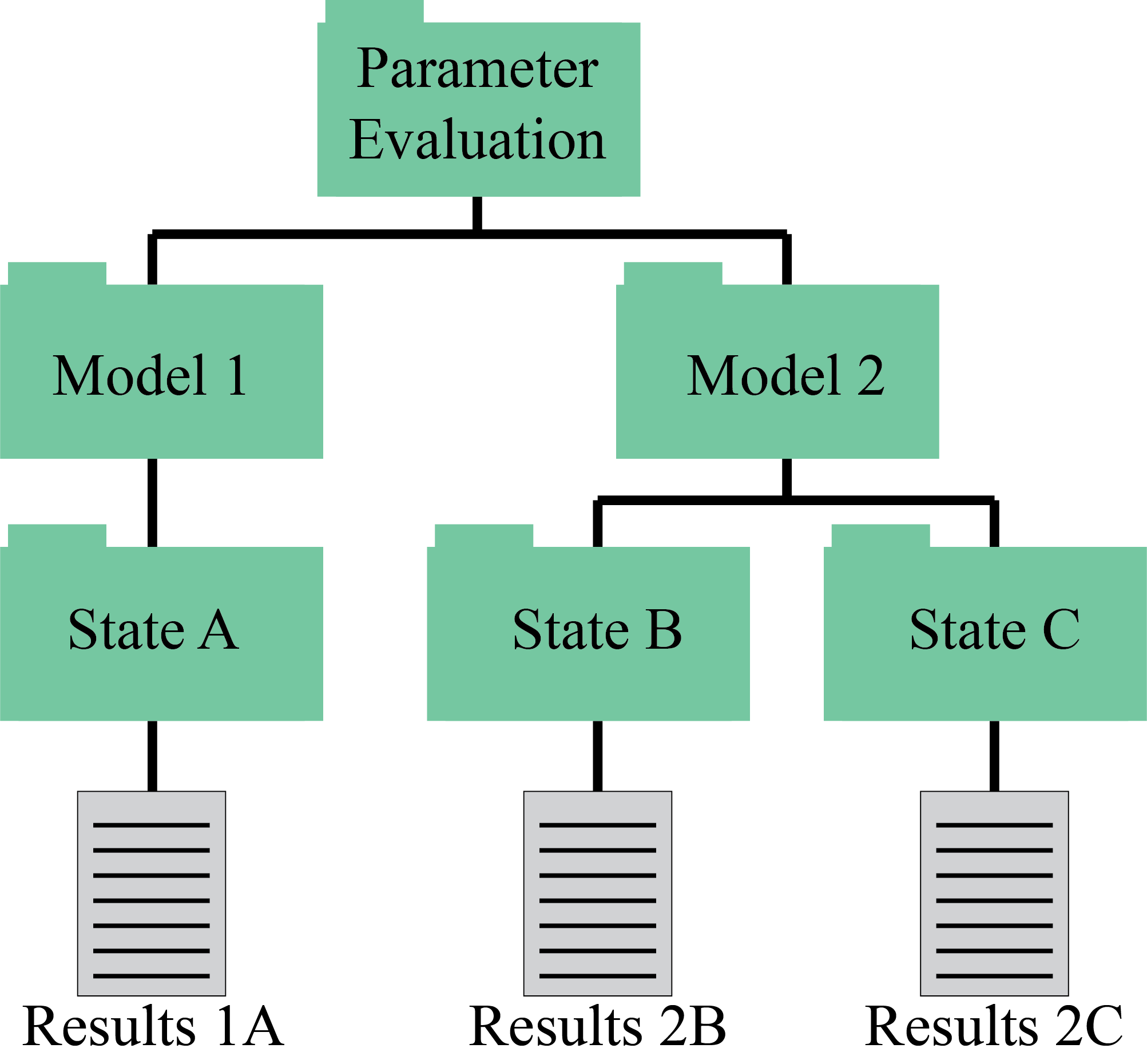
Fig. 1 File structure present in a given parameter set evaluation. Each model is evaluated at all states included in the data present in its evaluation set. The results of the model are found at the bottom of the tree.
However, in the calibration process we need to be careful when we have different counts of data from different sources. Having a larger number of data points in one set of data will bias the results to this data set. This is because that data set represents a larger contingency of the numbers that will be used to calculate the objective. To address this issue, MatCal normalizes all its residuals by the number of entries in the residuals.
This normalization means that if there is a ten percent error in a model prediction with 100 data points, then its evaluation generates the same magnitude of objective difference as if it had 1000 data points. To achieve this effect, the residuals are scaled by their data set size, the number of data sets in their state, and the number of states in the model. How these values are applied changes depending upon which objective definition is used. Most calibrations use something similar to an L2-norm, which requires that the residual be scaled by the square root of the terms listed above. This is shown in equation (3).
(3)
In our example if each data set had 16 entries,
the residual from results 1A would be scaled by
 and the residual from results
2B and 2C would be scaled by
and the residual from results
2B and 2C would be scaled by  .
.
Measuring
The last stage of the objective calculation in MatCal is
to convert the collection of weighted, normalized residuals
into a single objective.
The objective serves as an overall measurement of
the total disagreement between the experimental data and the model predictions.
For most calibrations in MatCal this is done using the Euclidean norm (L2-norm)
which is the default norm for most objectives.
Several norms are available including the L1-norm and all vector norms
supported by NumPy’s linalg.norm function. See
NormMetricFunction,
L1NormMetricFunction, and
L2NormMetricFunction
For this measurement, all the residuals from a given objective
set are concatenated
on top of each other to form a monolithic residual vector.
An objective set includes all residuals calculated for a study
as a result of adding an evaluation set to the study with
add_evaluation_set().
Note
Due to how we handle objectives in objective sets,
you will get a different number of objectives if you add multiple
objectives using a single call of
add_evaluation_set()
than you will if you add each on individually
with separate calls of
add_evaluation_set().
This will primarily affect algorithms that explicitly handle multiple objectives, but
will produce slightly different objectives for the same problem.
With the concatenated residual( ),
the objective(
),
the objective( ) is calculated by taking the appropriate norm
for the objectives. For the typical case of the L2-norm, this is the inner product of the
concatenated residual with itself, and then taking the square root of it(equation (4)).
) is calculated by taking the appropriate norm
for the objectives. For the typical case of the L2-norm, this is the inner product of the
concatenated residual with itself, and then taking the square root of it(equation (4)).
(4)
For problems with multiple objectives, the normalized values are summed to form a single objective. This is the value that most calibrations attempt to minimize. Some calibration methods will operate directly on the residual, in which the normalized, weighted residual is used by the calibration method to calibrate the material parameters. Even if the objective is not used for the calibration method directly, it is still calculated by MatCal and can be output using MatCal’s internal plotting tools to easily observe the convergence behavior of a particular calibration.
MatCal Models
This section covers the interfaces we provide for different models…
more coming soon
Python Models
Go over issues, such as need to be global and work with global variables if not MatCal parameters for pickling
User Executable Models
Add example - simple Python Model
Surrogate Models
Add example - building surrogate (might link)
MatCal Generated SIERRA Standard Models
Since material characterization tests are frequently standardized, we have developed a library of validated and maintained models that simulate a subset of these tests. Currently, only standard models for SIERRA Solid Mechanics have been developed.
These models have been peer-reviewed and used in calibrations found in the various MatCal examples. For code and model quality, these models are tested during each code update in MatCal’s unit and regression test suite. During production code releases, these models are tested in a larger suite of production tests to further ensure their accuracy and quality. Finally, the models are also validated against experimental data and, when possible, material models calibrated using these models are validated against validation experiments that typically use nonstandard test geometry. This provides implicit validation of the models, since they can be used to provide calibrated material models that accurately predict responses of validation experiments.
- MatCal SIERRA Solid Mechanics Standard Models
- Standard Model Geometry and Input Generation
- Simulation Coordinate Systems Available to the Material Model
- Simulation time control settings
- Simulation global output and access
- Simulation exodus output and settings
- Staggered and iterative coupling
- Overriding model parameters during a study
- MatCal Generated Models V&V Activities
Deriving Custom Model Classes
Data Importing and Manipulation
All MatCal calibrations and studies require data to which the models will be compared. MatCal has several custom tools for data importing and manipulation. In combination with what is available in Python, data can be imported, processed, analyzed and viewed quickly and easily.
Data Object Creation and Storage
First, data must be generated or imported from some
external source and stored in the appropriate
object. For MatCal, a single data set must
be stored in a Data object to
be used for most MatCal functions and tools.
A single data set is defined as group of measured quantities from a single
test or simulation. In MatCal, the measured quantities
are referred to as fields and each field has an associated field name.
The only requirement on the data is that the data fields must be the
same length. When the Data is
created in MatCal using its constructor or the
convert_dictionary_to_data() function no
checks on the data are made.
The Data
objects also have an optional attribute State.
The state for a data set is meant to store conditions or
metadata about the test that is necessary for
identification and needed for a simulation of the test.
Common state parameters include temperature and rate
for solid mechanics simulations. States are not
required for a data set but are used throughout
to inform model conditions when necessary and
pair model results appropriate with experimental
data. If none is assigned, MatCal will assign
its default empty state SolitaryState
to the data.
Data importing from external sources is supported
through valid MatCal data importers found
in data_importer. There are two primary tools
for data importing:
Importing data from single files using
FileData()function.Import data from several similar files with a filename regular expression using the
BatchDataImporterclass.
A useful class for storing several related
Data objects is
a MatCal DataCollection.
These data collections store data objects
by their states. For each state, the collection
can store multiple data objects. The intent
is that when storing experiment data, the collection
can store multiple repeat experiments for a given state.
The following code shows how to access the 4th
repeat data set for state “state_1” in a previously
created data collection “my_data_collection”:
my_data = my_data_collection["state_1"][3]
For more data manipulation examples, see Data manipulation.
Importing a single data set from a file
The FileData()
function will load CSV text files, NumPy arrays saved
using the NumPy array save method, or
MATLAB “.mat” files. The importer ensures
the data are integer or floating-point values and
then checks that all data are finite.
It will allow
string data if requested by the user with the
“import_strings” argument set to True. The imported
data are returned from the importer in the
MatCal Data format.
The name for the Data object is
set to the absolute file path of the file from
which it was loaded. The name is intended to be a
unique identifier for the data set which
may be important for data traceability.
States can be assigned to the data in three ways:
They can be passed as an argument through
FileData().It can be assigned to the
Dataobject through itsset_state()method.Alternatively, state parameters can be placed inside the file as dictionary for CSV file importing. This feature is described in detail in below.
CSV file data importing details
For CSV files in their simplest standard format,
the function expects
the first row that it reads to be the
field names and the following rows to
be the field values. Each column is dedicated
to a field and separated by a comma. It also
expects the files to have a “.csv” file extension,
although other file extensions can be read in if the file
type is specified as “csv” using the file_type argument.
More complex
CSV file formats are supported, and the importer
can read in state information from the file
and ignore any comments. Additionally, the
FileData()
function is a wrapper
for the NumPy “genfromtxt” function when used on CSV
files and can use most
valid “genfromtxt” keyword arguments passed to it.
Valid “genfromtxt” keyward arguments include:
comments
usecols
skip_footer
converters
missing_values
filling_values
When reading a CSV file, the function expects it to have the following structure:
{"state_param_1":value_1, "state_param_2":value_2, "state_param_3":"str_value_1"}
#
# Optional comments...
#
field_name_1, field_name_2, ..., field_name_n
 value[1, 1],  value[1, 1], ...,  value[1, n]
...
#
# Optional comments dispersed through data
#
...
 value[m, 1],  value[m, 1], ...,  value[m, n]
#
# More optional comments...
#
The first line is an optional dictionary
containing state information for the data. This dictionary
must have correct Python dictionary
syntax and valid MatCal state parameter names
and values or the state import will fail. If there
is no dictionary on the first line, the data
are loaded with the SolitaryState
default MatCal state with no state parameters.
After the dictionary, there can then be any
number of comments dispersed throughout
the file as long as the correct comment character
has been specified using the keyword argument
“comments”. For the file above,
the function call would look as follows:
my_data = FileData("csv_filename.csv", comments="#")
which sets the comment character to “#”. The next line to be read after removing the comments is the data header with the data field names followed by the field data values. All rows that are read in must have the same number of columns.
For the file above, the data will
be imported with the N field names and will
have three state parameters “state_param_1”,
“state_param_2” and “state_param_3” with the appropriate
values for its assigned State.
The name for the state is automatically assigned as
“state_param_1_value_1_state_param_2_value_2_state_param_3_str_value_1”.
The numeric state values are formatted in scientific notation
with a precision equal to six when the name is generated.
NPY and MAT file data importing details
For “.npy” files, the data importer
expects that the data are stored
as a structured array so that
the data types have names which will become
Data objects
the field names. The data associated with each field
can be an array of any dimension.
For MATLAB “.mat” files, the
data structure variable names will become the field names for
the MatCal Data object
and all fields are expected to be one dimensional vectors.
Importing data from a list of filenames or a regular expression
The BatchDataImporter class
imports multiple files of a common file type into
a DataCollection. In its
simplest use case, it imports all data and assigns them
all a common state
State.
For an import with no state information,
data are assigned
the MatCal default SolitaryState state.
If the “fixed_states” argument is passed to the class
constructor, then the data are assigned
a state named “batch_fixed_state” with the dictionary keyword/value
pairs from “fixed_states” assigned to them as state parameters.
The import for each file in the batch
is done using the FileData()
function and supports its file types and limitations.
As a result, if all files are CSV files and have states defined in
the files using a dictionary as the first line,
then the batch importer will store them by those states in
a DataCollection it builds and returns with its
batch() method.
The batch importer can also combine similar states into
a single state if desired. Frequently experiments will have target states,
but the specific value of the state for a given test will
fluctuate with some error. For example, an experiment
may be nominally testing a material at 500K. However,
over three repeats the initial temperatures were measured
at 498K, 502K, and 505K. To treat these as individual
states in a calibration or other study
would require running
the model three separate times since MatCal
evaluates all data states for model when comparing it to that data.
If the difference is negligible, the added computational
cost of running each state may not be acceptable.
It may be desirable and beneficial, to assign these
the state value of 500K the target temperature for
the test. This can be done by setting the
“state_precision”=1 option for the batch importer
using the set_options
method. Currently, “state_precision” is the only option
that can be specified. An example input for loading
data with a batch import is below:
my_batch_importer = BatchDataImporter("test_data*.txt", file_type="csv")
my_batch_importer.set_options(state_precision=1)
my_test_data_collection = my_batch_importer.batch
Data manipulation
Data manipulation is a vital preprocessing step
when preparing raw experimental data for a
calibration or other MatCal study. With this in mind,
the Data class
is derived from NumPy arrays [7] and
can be manipulated using most NumPy array tools. In addition,
for both Data and
DataCollection we added a few
methods to aid in manipulation.
The most useful features for data manipulation
in MatCal are NumPy’s slicing features.
For a Data slicing
can be used to down sample or select subsets of
the data. For example, if data have the
field names “time”, “load”, “displacement”, “temperature”
with 100,000 points in each field, you may want to
down sample the data for memory reason and
select only the fields needed for the study.
We will start by removing the unnecessary fields.
Let’s assume that we do not want to use the “time”
field. It can be removed using slice as shown
below:
data = data[["load", "displacement", "temperature"]]
where the “time” field is not included in the requested fields from the data. In this case the data overwrites itself effectively removing the “time” field from the data object. Another less manual way to remove fields is:
data_fields = data.field_names
data_fields.remove("time")
data = data[data_fields]
The above is what is done when using the data
remove_field() method.
Continuing this example, we wish to purge data
from the data object with displacements less than zero
and down sample it to around 1000 points. Once
again, we use slicing to do so:
data = data[data["displacement"] >= 0]
desired_data_len = 1000
interval = int(len(data)/desired_data_len)
data = data[::interval]
which produces the desired result and stores it back in “data”.
Another useful set of
features that Data
inherits from NumPy arrays are all the
math operators that can act on arrays.
An example of applying simple scaling and offsets to the data for
general data manipulation is below.:
from copy import deepcopy
data_scaled = deepcopy(data)
data_scaled["displacement"] *= 25.4 # scale from inches to mm
data_scaled["load"] -= 100 #shift the load down by a value of 100.
To see more NumPy operators or features that may be of use, please visit the NumPy documentation on arrays.
The last Data method
that can be particularly useful when importing data from
different sources is the remove_field() method.
It can be used to give a field a new name. When
using MatCal Generated SIERRA Standard Models, this
may be required to ensure the correct fields exist in the
data for boundary condition generation and objective function
calculation. An example of using this method is:
data.rename_field("old_name", "new_name")
field_data=data["new_name"]
and the previously named “old_name” field is now accessed using the “new_name” field name.
MatCal’s DataCollection
class also has a few data manipulation methods and tools
available for users. These features simplify
some of the manipulations above specifically for
data collections. Since data collections are larger,
nested structures for data, manipulation can be more difficult
due to the layers that must be navigated to access data.
The following tools are available:
The
remove_field()method for data collections which behaves similarly to the method forData, but acts on all data set held in the data collection.The
plot()method which will plot data from a data collection when an independent and dependent field is passed to the method. It plots the data on a 2D plot with each state on a separate figure.The
scale_data_collection()function that can be used to apply scales and offsets to all data sets in a data collection that have the field name requested for scaling. It returns a new scaled data collection and does not modify the data collection passed to it.
Examples of these data manipulation features being used for both data preprocessing and objective function residual weighting can be found here Successful Calibration and here 304L stainless steel viscoplastic calibration
Full-field Data Specific Features
Note
Full-field data is currently intended to be only be used on nearly planar two-dimensional surfaces. MatCal’s Virtual Fields Method is strictly limited to two-dimensional data. Technically, MatCal’s Full-field Interpolation and Extrapolation and Hierarchical Wavelet Decomposition methods can be used with non-planar surfaces as long as the points are uniquely identified by a given two-dimensional set of spatial cooridnates, e.g. “X” and “Y” pairs.
Extensions to three-dimensions are planned for future releases.
We simplifiy full-field data manipulation and importing by providing
an importer that works with common file formats.
The FieldSeriesData() imports field data from CSV
and exodus files into MatCal. This function stores full-field data and
its associated global data in
a single FieldData object that
supports all functions of the Data
objects but has a few specific full-field data specific attributes.
Since it is derived from the Data class,
it can be used in most MatCal functions and classes that
operate on Data objects.
FieldData objects can also be manipulated
as described in Data manipulation for any of their data
fields. For field data an important added attribute is the
spatial_coords. These hold the
reference configuration coordinates for the data held in
the FieldData objects.
Except for the spatial_coords,
all other field data is stored in two-dimensional arrays that
can be accessed from the FieldData object
using the field name. The rows of the accessed two-dimensional
array correspond to each time step and the data in each
column corresponds to each point. The indices for each column
should match accross field in the stored field data by time step.
When accessing the reference configuration spatial coordinates
from spatial_coords, a
single two dimensional array is returned where the columns
correspond to the “position_names” arguments passed to
FieldSeriesData() and
the rows correspond to the number of points. The row
indices for the spatial coordinates
correspond to the column indices in the field data
fields that vary with time for a point. For example,
the following block of code gets the reference configuration
position and displacement for the same point from a
FieldData object.:
my_field_data = FieldSeriesData("field_data_global.csv")
point_position_of_interest = my_field_data.spatial_coords[101, :]

#point_position_of_interest now stores the X/Y postion of point 101
point_x_displacement_of_interest = my_field_data["X"][:, 101]
point_y_displacement_of_interest = my_field_data["Y"][:, 101]

point_x_deformed_position = point_position_of_interest+point_x_displacement_of_interest
point_y_deformed_position = point_position_of_interest+point_x_displacement_of_interest
Warning
Performing data manipulation, such as slicing on, the data fields in a
FieldData object
will not also be applied to the spatial coordinates. You will
need to perform similar manipulations on the spatial coordinates
to get the desired results. This due to the fact that
field data for a given field, e.g. “u” for x displacement, is
expected to be a two-dimensional array where the rows correspond to each time
step and the columns correspond to each point where the field
data is recorded. Since spatial coordinates are constant through
time, they are stored as one-dimensional vectors and the slices
used on the fields may not apply. Perform the appropriate
equivalent slice on the spatial coordinate data and then update it
in the FieldData object using
set_spatial_coords().
Full-field Data Importing from CSV
Using FieldSeriesData() has some
notable differences when importing CSV data when compared to the
FileData() function.
For CSV data, you must point to a global file that contains
any global data of interest such as “time”, “load” or “displacement”.
The global file is required to have a field named “file”
that can be in any column. The “file” field contains the filename
of other CSV files that contain all of the relevant field data for
each time step. For example, the global data CSV file
for a series of CSV files of field data would look
similar to:
#
# Optional comments...
#
global_field_name_1, ..., global_field_name_n, ..., file
 value[1, 1],  ..., value[1, ], ..., field_filename_time_step_1
...
#
# Optional comments dispersed through data
#
...
 value[m, 1],  ..., value[m, n], ...,  field_filename_time_step_m
#
# More optional comments...
#
Note
Currently, FieldSeriesData() will
not read state data from the files. The state information has to
be passed as the “state” keyword argument to
FieldSeriesData() or can be set
using set_state()
The files that contain field data listed in the “file” field of the
global data file should look like a typical CSV data file
that is read in using the FileData()
function as documented in CSV file data importing details. Their
path that is specified in the “file” field can be absolute or
relative with respect to the path specified in the “series_directory”
keyword argument to FieldSeriesData().
As with the global file, any state information at the top of the time step
data files are
ignored. The spatial_coords are set
from the data in the first file provided in the global filename list
under the “file” field. The coordinates are imported from the data
fields named according to the “position_names” keyword argument in
FieldSeriesData(). They default
to “X” and “Y”, but the “position_names” keyword argument will
accept a list or tuple of two strings that are valid keys
in the data file containing the first time step field data.
A useful argument for importing large data sets from CSV is the “n_cores” argument.
It allows a parallel read of file data using subprocesses. The full data object is built
on the parent thread in serial, but reading the files on separate processes
has shown to reduce the data importing time for CSV files to
about half of the time loading them in serial. Building the full
FieldData object in parallel
is currently not supported because it cannot benefit
from parallelization due to Python’s Global Interpreter Lock.
Full-field Data Importing from Exodus
The FieldSeriesData()
function uses ExodusPy to read in data from an
exodus mesh results file. It currently ignores
the “series_directory” and “n_cores” keyword
arguments when importing data. It will load
decomposed mesh files as long as the base filename
for the decomposed mesh files is the same
as that passed as the “global_filename” argument
to the function. When opening a decomposed set
of files it uses the Seacas tool EPU to
reconstruct the decomposed mesh into a single
mesh. True parallel reads are not currently supported.
Every time step, node variable and element variable are
loaded into the FieldData object.
These can then be accessed through the field names
and array slicing if necessary.
Warning
If using full-field data tools with your own model, make
sure to only output variables and time steps that are needed
for the study being performed.
When importing the exodus data, the FieldSeriesData()
stores all available data in memory and large results files can
quickly result in out-of-memory errors.
Generally, the user is not expected to import data from exodus files unless they are perfoming studies on synthetic data. However, for studies using Sierra models with full-field objectives, all of MatCal expects results to be in exodus format.
Results and Plotting
MatCal has a few tools to help users manage, view and manipulate all the model results created through a MatCal study.
Plotting
The primary tool for results viewing is the “plot_matcal” plotting utility. It should be available for command line execution after loading a “matcal” module on a computing resource where MatCal is installed. It currently creates three types of plots when called:
The simulation QoIs along with the experimental data QoIs.
The objective value as a function of the evaluation number.
The objective value as a function of each parameter.
By default, the objective plots are created only for the total objective which is a combination of all evaluation set objectives. If you want to plot each objective independently, use the “–plot_model_objectives”/”-pmo” option. The QoI plots are created for all model and experiment QoI sets added as evaluation sets. In addition, for the simulation and experiment QoIs, a plot will be created for each state, since the results for each state may have much different maximum and minimum bounds. By default, all images are displayed after the plotting function has been called. To run the plotting script from the command line using the following:
plot_matcal -i "independent_field_1,independent_field_2,...,independent_field_n"
where independent_field_1 through
independent_field_n are valid
independent field names for the data sets contained in the model objectives.
These independent fields specify all fields that will be used as independent
fields on the horizontal axes of the QoI plots. All remaining fields available in the objectives
will be plotted as dependent fields on the vertical axes of the plots.
This command must be run in the directory where MatCal is running and
reads results from the *.joblib files created by MatCal
which stores study results as the studies run.
Warning
For large studies,
this can result in many figures.
A --no-show will be available in future releases
to suppress showing images.
Since model and experiment QoIs from all objectives will be plotted when using this command, a valid field name must be given for each objective when specifying desired independent fields or the plotting script will fail. Another option is to pass no independent fields. In this case, all fields will be plotted as both the dependent and independent field for the QoI plot, creating an NxN table of subplots where N is the number of fields in the results data.
The make_standard_plots() can
be called from a python interactive shell or a python script to
make the same plots. See its documentation for use.
Example showing results created with the plotting script are 304L stainless steel viscoplastic calibration and Successful Calibration.
Results Data and Output
Results output from MatCal studies currently comes in several forms with some dependence on the type of study being performed. For all MatCal studies, there are at least three different ways to access study results.
The results object returned from the
launch()method.The “in_progress_results.joblib” and “final_results.joblib” files store the entire evaluation history from all completed parameter batches. The in progress results stores results up to and including that last evaluated parameter set batch. It is replaced by the final results file at the end of the study which includes the entire parameter evaluation history. Both files store a
StudyResultsobject.The MatCal log file which contains objective information for all evaluated parameters and any errors or output from the underlying study.
Depending on the type of study, a best material parameter file may also be written. It will contain Aprepro [28] style variables or a dictionary with the values taken from the evaluation with the lowest objective from all parameter sets that were evaluated during the study. Output is dependent on how MatCal is setup for your platform.
For Dakota based studies, additional output includes:
The “dakota.out”, “dakota.err” and “dakota_tabular.dat” files written by Dakota. The verbosity of output written to “dakota.out” can be controlled by the
set_output_verbosity()method called on a Dakota study.The “dakota.rst” files used to provide restart information for a Dakota based study.
Any additional output files produced by Dakota’s libraries.
MatCal is designed such that users should interact with the files output by MatCal and the results object returned from the study.
Note
The evaluation name is also the folder name that the models for the evaluation are run in if their simulations require an external executable.
The results object contains significant data related to the objective
calculation which includes the simulation/experiment QoIs, the
residuals and the objective values calculated from the residuals for each
evaluation.
It also includes the entire parameter history and the names
for each evaluation in the history. To access the results from the files written
to disk use the matcal_load() function
with the appropriate results filename passed to it.
Warning
The specifics stored in the results files may change over time. We are still working to determine what should be stored in these objects; however, we will attempt to keep the objects backward compatible.
Always refer to the API documentation for
matcal_load()
and StudyResults to get the most
up-to-date structure for the files returned from the functions.
The results output from the study launch() method
will return a the same StudyResults
as is saved to disk. The results saved from different studies
will likely have different attributes specific to that study.
See the API documentation for specifics on the returns from different studies.
For Dakota calibrations, the most relevant returned result is the calibrated parameter sets.
In the results dictionary returned from these studies these are accessed with the
under the “best” attribute using “results.best”.
The examples are also a good reference for how to access and use results data for post-study analysis, results plotting or follow-on studies. The Introduction Examples include most study types, and demonstrate how to manipulate the output data from some of these studies.
Options for Parallel Computing
In MatCal, the use of parallel processing is supported in several ways.
The primary methods involve how many processes can be used by a model and
how many processes a study is limited to use as a maximum through out the study.
The former is set using set_number_of_cores()
and the latter is set using set_core_limit().
Model set_number_of_cores method
First, we will describe specifics of the set_number_of_cores method.
This method is valid for all MatCal models. The value passed to set_number_of_cores
is how many cores the job will use to
execute one evaluation of the model.
Note
The PythonModel and the
UserExecutableModel do not actually enforce the use
of the number of cores. MatCal just uses this for calculating how many cores are currently
in use when these models are run. The user is expected to control how the models are run in parallel
through their use provided functions or files.
For MatCal Generated SIERRA Standard Models, MatCal passes the number of cores to SIERRA which runs the model on that many processes. This number should be strictly enforced.
Study set_core_limit method
The set_core_limit method for MatCal Studies sets a hard limit to how many
cores can be used by models run by the study. Since many MatCal Studies
can evaluate objectives for different parameter sets concurrently and a single parameter
evaluation may require the execution of several models, this is used to ensure
that the available processes or cores on a machine is not oversubscribed.
For example, if a study needs to evaluate 10 models for a single objective and 10 parameter set values
for a given parameter batch, it would run 100 models concurrently for maximum parallelism. However,
if each model uses 5 cores and the available cores on the machine where the study is run is 32,
then it is not possible to run all 100 models concurrently. If 15 was passed to set_core_limit,
then three models would be run concurrently. A new one would be started every time one finished
until all 100 models for the current parameter set batch completed for the study and a new
parameter set batch was determined by the study algorithm so that it could continue.
The previous paragraph describes how this works when all models are run on
the same computing platform or node as the study. However,
on high performance computing platforms, jobs may be run on different nodes or
even on remote platforms through a queueing system. When a model is set to run in this
way using matcal.core.models.UserExecutableModel.run_in_queue(), then the model
only counts as the study using one processes when the the study enforces the
study core limit even if the model uses more than one core. This is because the
cores for the model are not loading the machine where the study is being run. The study
just needs to account for a single process for job monitoring and results processing.
Note
Once again, the PythonModel and the
UserExecutableModel do not actually submit the
jobs to the queueing system. The user is expected to do so within
files and functions supplied for these models.