Objective Sensitivity Study

In this example, we perform a sensitivity study where we observe how several objectives vary as we change the material parameters by +/- 5% from the values used to generate the synthetic data. We do this for only one data set, the 0_degree data set, because we wish to gauge whether it is possible to calibrate all parameters to one data set.

We are going to assess the sensitivity of five objectives to the input parameters:

1. The CurveBasedInterpolatedObjective for the load-displacement curve.

2. The InterpolatedFullFieldObjective for the X and Y displacements.

3. The PolynomialHWDObjective without point colocation.

4. The PolynomialHWDObjective with point colocation.

5. The MechanicalVFMObjective used with the VFMUniaxialTensionHexModel.

To begin, we import the MatCal tools necessary for this study and import the data that will be used for the calibration.

from matcal import *
import numpy as np

Next, we import the data we wish to use in the study. For this study, we must import the same data set twice. This is because we need to have displacement named something other than “displacement_(x,y,z)” for the VFM model and the other model will need to compare to “displacement_(x,y)” for their objective. We could also output displacement as another name from SierraSM, but then some visualization software would not automatically load the deformed configuration. Renaming fields and importing the data twice is simple with MatCal’s Data Importing and Manipulation Tools.

synthetic_data = FieldSeriesData("../../../docs_support_files/synthetic_surf_results_0_degree.e")
synthetic_data.rename_field("U", "displacement_x")
synthetic_data.rename_field("V", "displacement_y")
synthetic_data.rename_field("W", "displacement_z")

vfm_data = FieldSeriesData("../../../docs_support_files/synthetic_surf_results_0_degree.e")

Opening exodus file: ../../../docs_support_files/synthetic_surf_results_0_degree.e
Opening exodus file: ../../../docs_support_files/synthetic_surf_results_0_degree.e
Closing exodus file: ../../../docs_support_files/synthetic_surf_results_0_degree.e
Closing exodus file: ../../../docs_support_files/synthetic_surf_results_0_degree.e
Opening exodus file: ../../../docs_support_files/synthetic_surf_results_0_degree.e
Opening exodus file: ../../../docs_support_files/synthetic_surf_results_0_degree.e
Closing exodus file: ../../../docs_support_files/synthetic_surf_results_0_degree.e
Closing exodus file: ../../../docs_support_files/synthetic_surf_results_0_degree.e

After importing the data, we select the data we want to use for our study. For the load-displacement curve objective, we want all time steps up to 92.5% of the peak load past peak load. These data are selected for the synthetic_data object below. For the HWD and interpolate full-field objectives, we select only three time steps. One is early in the load-displacement history, the second is at peak load, and the third is at 92.5% of peak load past peak load. We call this truncated data selected_data. The final vfm_data contains all data before peak load where VFM is valid.

peak_load_arg = np.argmax(synthetic_data["load"])
last_desired_arg = np.argmin(np.abs(synthetic_data["load"]\
                                    [peak_load_arg:]-np.max(synthetic_data["load"])*0.925))
synthetic_data = synthetic_data[:last_desired_arg+1+peak_load_arg]
synthetic_data.set_name("0_degree")

last_disp_arg = np.argmax(synthetic_data["displacement"])
selected_data = synthetic_data[[200, peak_load_arg, last_disp_arg]]
selected_data.set_name("selected data")

vfm_data = vfm_data[vfm_data["displacement"] < 0.036]

With the data imported and selected, we plot the data to verify our data manipulations.

dc = DataCollection("synthetic", synthetic_data, selected_data)
dc.plot("displacement", "load")
import matplotlib.pyplot as plt

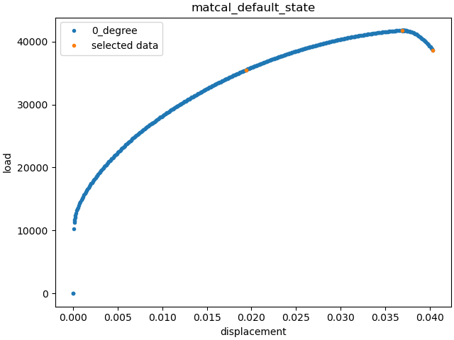
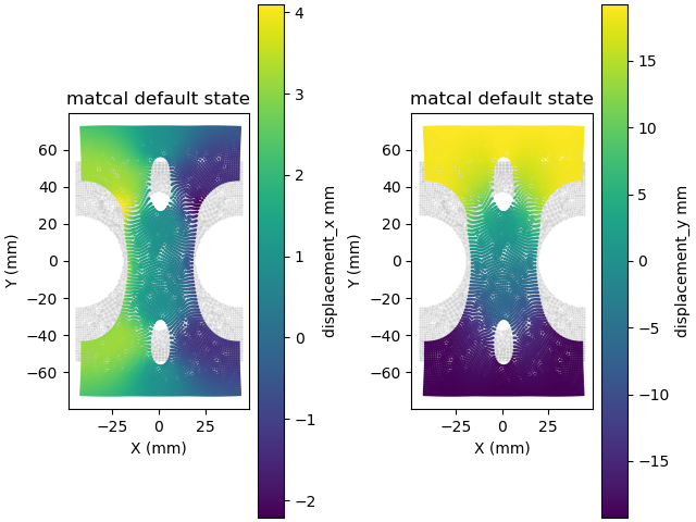
Above, we can see the data we selected in orange and verify these are the points of interest. Next, we plot the displacement fields. We plot the deformed configuration colored according the correct displacement field on top of the undeformed configuration in grey.

def plot_field(data, field, ax):
    c = ax.scatter(1e3*(data.spatial_coords[:,0]),
                   1e3*(data.spatial_coords[:,1]),
                   c="#bdbdbd", marker='.', s=1, alpha=0.5)
    c = ax.scatter(1e3*(data.spatial_coords[:,0]+data["displacement_x"][-1, :]),
                   1e3*(data.spatial_coords[:,1]+data["displacement_y"][-1, :]),
                   c=1e3*data[field][-1, :], marker='.', s=3)
    ax.set_xlabel("X (mm)")
    ax.set_ylabel("Y (mm)")
    direction = data.state.name.replace("_", " ")
    ax.set_title(f"{direction}")
    ax.set_aspect('equal')
    fig.colorbar(c, ax=ax, label=f"{field} mm")

fig, axes = plt.subplots(1,2, constrained_layout=True)
plot_field(synthetic_data, "displacement_x", axes[0])
plot_field(synthetic_data, "displacement_y", axes[1])
plt.show()

After importing and preparing the data, we create the models that will be used to simulate the characterization test. We will make both a UserDefinedSierraModel and a VFMUniaxialTensionHexModel for this example. Both of these models will need the same SierraSM material model input file. We create it next using Python string and file tools.

mat_file_string = """begin material test_material
  density = 1
  begin parameters for model hill_plasticity
    youngs modulus  = {elastic_modulus*1e9}
    poissons ratio  = {poissons}
    yield_stress    = {yield_stress*1e6}

    hardening model = voce
    hardening modulus = {A*1e6}
    exponential coefficient = {n}

    coordinate system = rectangular_coordinate_system

    R11 = {R11}
    R22 = {R22}
    R33 = {R33}
    R12 = {R12}
    R23 = {R23}
    R31 = {R31}
  end
end
"""

with open("modular_plasticity.inc", 'w') as fn:
    fn.write(mat_file_string)

With the material file created, the models can be instantiated. We start with the UserDefinedSierraModel and point it to the correct user-supplied input deck and mesh. For this model, we use adagio as the solid mechanics simulation code. We use the appropriate model methods to set up the model for the study. Most importantly, we pass the correct model constants to it and tell the model to read the full field data results from the output exodus file.

model = UserDefinedSierraModel("adagio", "synthetic_data_files/test_model_input_reduced_output.i",
                               "synthetic_data_files/test_mesh.g", "modular_plasticity.inc")
model.set_name("3D_model")
model.add_constants(elastic_modulus=200, poissons=0.27,
                    R22=1.0, R33=0.9, R23=1.0, R31=1.0)
model.read_full_field_data("surf_results.e")

from site_matcal.sandia.computing_platforms import is_sandia_cluster, get_sandia_computing_platform
from site_matcal.sandia.tests.utilities import MATCAL_WCID
num_cores=96
if is_sandia_cluster():
    platform = get_sandia_computing_platform()
    num_cores = platform.get_processors_per_node()
    model.run_in_queue(MATCAL_WCID, 0.5)
    model.continue_when_simulation_fails()
model.set_number_of_cores(num_cores)

The VFM model requires a Material object. After creating the material object, we create the VFM model with the correct surface mesh that corresponds to our output surface mesh and the total specimen thickness. Similar to the previous model, we use the correct methods to prepare the model for the study.

material = Material("test_material", "modular_plasticity.inc", "hill_plasticity")
vfm_model = VFMUniaxialTensionHexModel(material,
                                       "synthetic_data_files/test_mesh_surf.g",
                                       0.0625*0.0254)
vfm_model.add_boundary_condition_data(vfm_data)
vfm_model.set_name("vfm_model")
vfm_model.set_number_of_cores(36)
vfm_model.set_number_of_time_steps(450)
vfm_model.set_displacement_field_names(x_displacement="U", y_displacement="V")
vfm_model.add_constants(elastic_modulus=200, poissons=0.27, R22=1.0,
                        R33=0.9, R23=1.0, R31=1.0)
if is_sandia_cluster():
    vfm_model.run_in_queue(MATCAL_WCID, 10.0/60.0)
    vfm_model.continue_when_simulation_fails()

Opening exodus file: synthetic_data_files/test_mesh_surf.g
Closing exodus file: synthetic_data_files/test_mesh_surf.g

The objectives that we wish to evaluate are created next. All full-field objectives are given the correct input parameters to function correctly for the planned study. Primarily, this the mesh that they will interpolate the experiment data onto and the fields that will be compared.

interpolate_objective = InterpolatedFullFieldObjective("synthetic_data_files/test_mesh_surf.g",
                                                       "displacement_x",
                                                       "displacement_y")
interpolate_objective.set_name("interpolate_objective")

hwd_colocated_objective = PolynomialHWDObjective("synthetic_data_files/test_mesh_surf.g",
                                                 "displacement_x",
                                                 "displacement_y")
hwd_colocated_objective.set_name("hwd_colocated_objective")

Opening exodus file: synthetic_data_files/test_mesh_surf.g
Closing exodus file: synthetic_data_files/test_mesh_surf.g

A special case is the PolynomialHWDObjective, where the first input argument is None. The first argument is the mesh or point cloud that the fields will be mapped to. If None is passed, no interpolation is performed, and standard HWD without co-location is used. This should only be done for cases where the simulation mesh has its surface area completely within the experimental data. Otherwise, the objective will likely be invalid.

hwd_objective = PolynomialHWDObjective(None, "displacement_x",
                                       "displacement_y")
hwd_objective.set_name("hwd_objective")

load_objective = CurveBasedInterpolatedObjective("displacement", "load", right=0)
load_objective.set_name("load_objective")

vfm_objective = MechanicalVFMObjective()
vfm_objective.set_name("vfm_objective")

We then create the material model input parameters for the study with the initial point being the values used to generate the synthetic data, or the “truth” values.

Y = Parameter("yield_stress", 150, 250.0, 200.0)
A = Parameter("A", 1250, 2000, 1500.0)
n = Parameter("n", 1, 4, 2.00)
R11 = Parameter("R11", 0.8, 1.1, 0.95)
R12 = Parameter("R12", 0.7, 1.1 , 0.85)

param_collection = ParameterCollection("Hill48 in-plane", Y, A, n, R11, R12)

The ParameterStudy is created, and all evaluation sets are added.

Note

MatCal will only run the 3D_model once even though it is added multiple times. Only the extra objectives will be added to the additional evaluation sets.

study = ParameterStudy(param_collection)
study.add_evaluation_set(vfm_model, vfm_objective, vfm_data)
study.add_evaluation_set(model, load_objective, synthetic_data)
study.add_evaluation_set(model, interpolate_objective, selected_data)
study.add_evaluation_set(model, hwd_objective, selected_data)
study.add_evaluation_set(model, hwd_colocated_objective, selected_data)
study.set_working_directory("objective_sensitivity_study", remove_existing=True)

Opening exodus file: synthetic_data_files/test_mesh_surf.g
Closing exodus file: synthetic_data_files/test_mesh_surf.g
Opening exodus file: synthetic_data_files/test_mesh_surf.g
Closing exodus file: synthetic_data_files/test_mesh_surf.g

Since the processing of full-field data can be computationally expensive we limit the number of jobs that can be processed concurrently. By setting the core limit to 10, when run on a cluster only 10 models will be run and post-processed concurrently.

study.set_core_limit(10)

Since this study is evaluating many responses with full-field data, we reduce what is stored in the results objects to limit the amount of memory consumed in results storage. We are only interested the objectives as a function of the parameters and the different model responses. As a result, we only store the qois and objective values in the results object as shown below.

study.set_results_storage_options(data=False, qois=True, residuals=False, objectives=True)

The final step is to add the parameter values to be evaluated. First, we add the truth values, which should be the minimum for all objectives. Next, we add 10 values from -5% to +5% for each parameter. Only one parameter is varied at a time to simplify visualization. The function below adds the parameter evaluations to the study.

study.add_parameter_evaluation(**param_collection.get_current_value_dict())
evaluations = []
import copy
for name, param in param_collection.items():
    for val in np.linspace(param.get_current_value()*0.95,param.get_current_value()*1.05, 10):
        current_eval = copy.copy(param_collection.get_current_value_dict())
        current_eval[name]=val
        evaluations.append(current_eval)
        study.add_parameter_evaluation(**current_eval)

Next, we launch the study and plot the results.

results = study.launch()

Opening exodus file: matcal_template/vfm_model/matcal_default_state/vfm_model.g
Closing exodus file: matcal_template/vfm_model/matcal_default_state/vfm_model.g
Opening exodus file: matcal_template/vfm_model/matcal_default_state/vfm_model.g
Closing exodus file: matcal_template/vfm_model/matcal_default_state/vfm_model.g
Opening exodus file: matcal_template/vfm_model/matcal_default_state/vfm_model.g
Closing exodus file: matcal_template/vfm_model/matcal_default_state/vfm_model.g
Opening exodus file: matcal_template/vfm_model/matcal_default_state/vfm_model.g
Opening exodus file: matcal_template/vfm_model/matcal_default_state/vfm_model_exploded.g
Closing exodus file: matcal_template/vfm_model/matcal_default_state/vfm_model_exploded.g
Closing exodus file: matcal_template/vfm_model/matcal_default_state/vfm_model.g

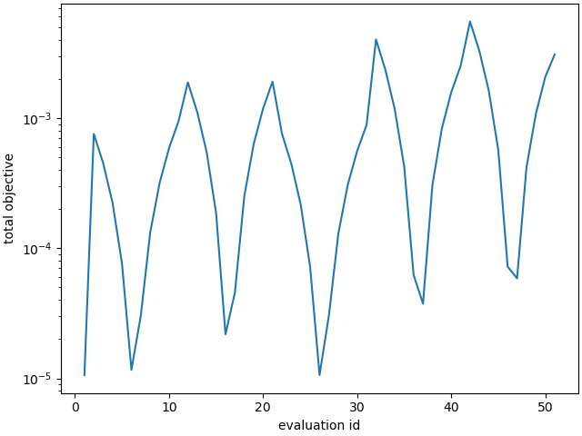
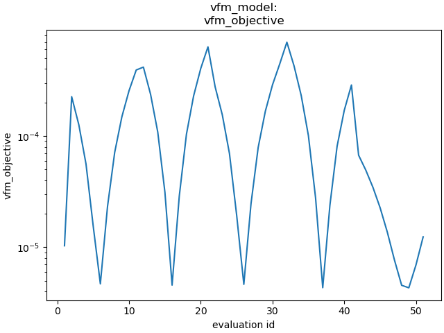
Several plots are output below, and we summarize the results here.

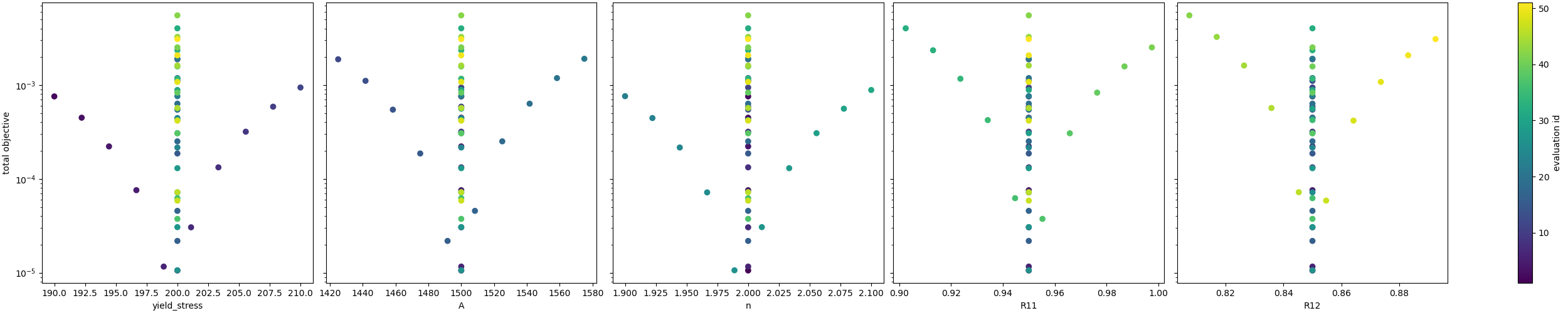
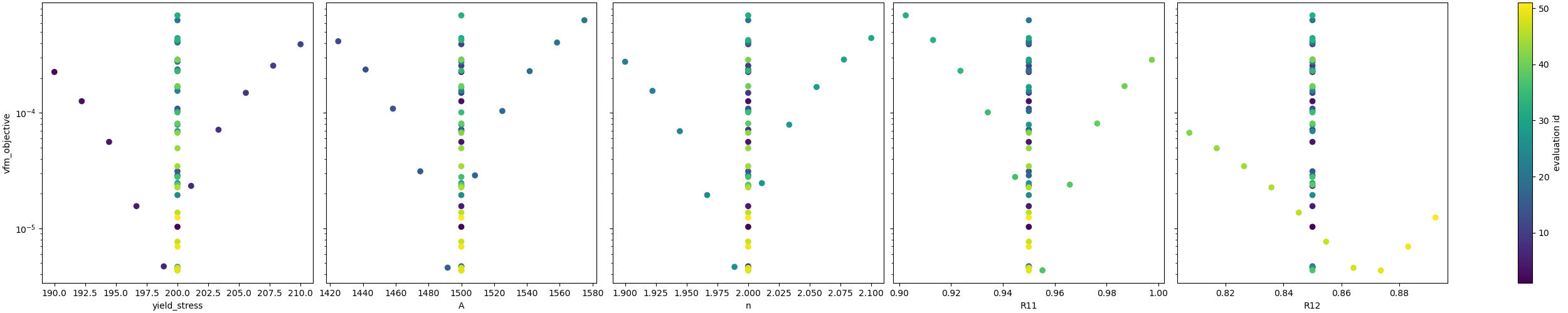
1. VFM objective observations: The first plot shows the VFM objective plotted for each parameter evaluation. As the input parameters change the objective increases and decreases smoothly with well defined local minima. One issue is that the first parameter set evaluated, which corresponds to the values used to generate the synthetic data is not the lowest. This is due to the model form error introduced by the plane stress assumption, and is expected. The shift in the global minimum is most obvious in the third plot, which shows how the objective varies with input parameters. The vertical lines of evaluations are the changes of the other parameters and should be where the global minimum is located. However, for each parameter, there exists at least one different local minimum that shifted slightly to one side in the parameter space from the expected minimum. The actual global minimum is likely somewhere else within the multi-dimensional objective function space.

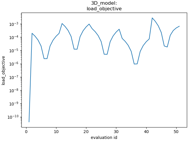
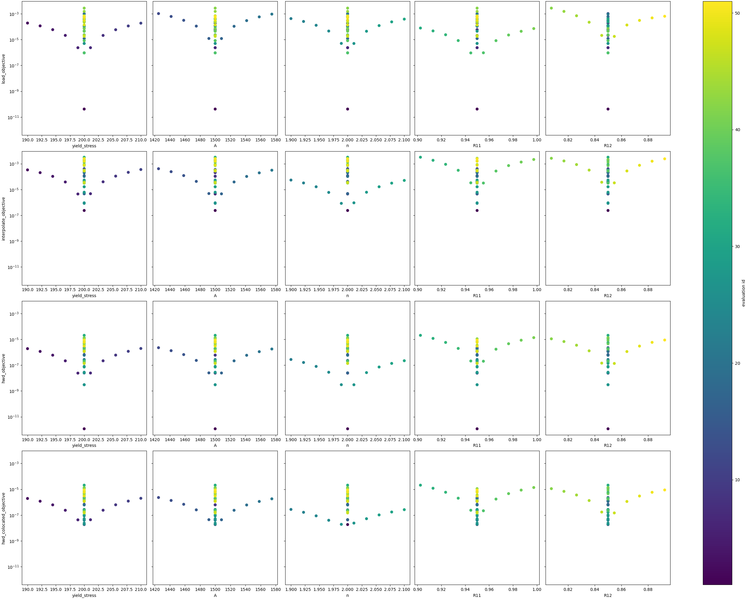
2. Load-displacement objective observations: The upper right subplot, for the second image, shows how the load-displacement objective changes with the parameters. It has a clear minimum at the expected global minimum at the first parameter evaluation. Overall, the objective is less smooth than the VFM objective across all evaluations. The first subplot of the fourth figure shows the objective sensitivity to the individual parameters. Here, again, the minimum is at the expected global minimum. One issue for calibration is that the objective has a what seems like a discontinuity or at least a sharp drop to the right and left of the minimum. This sharp change in the objective will be problematic for gradient methods and is likely more complex in the full five-dimensional space of the objective.

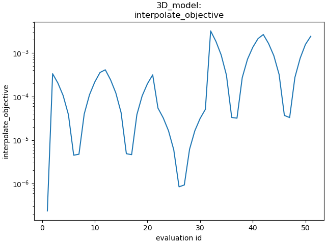
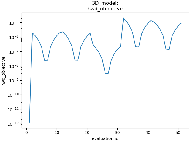
3. Full-field interpolation and HWD objective observations: The HWD objective without point colocation and the full-field interpolation objectives produce similar results. This is expected, as the HWD objective is a linear transform of the displacement field and is a very similar comparison. The objective values for the methods as a function of parameter evaluation are shown in the top right and bottom left of the second figure. Both figures show the same general objective landscape with their minima at the expected global minimum. There are two noticeable differences: (1) the HWD objective has a lower overall magnitude since the normalization routine scales the objective slightly differently and (2) there is a much lower objective at the expected global minimum for HWD. The high objective values for the interpolation method at the global minimum is due to small errors introduced by interpolation.

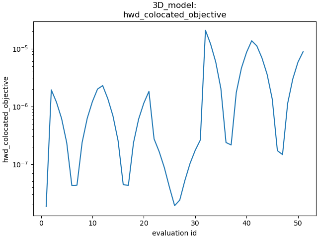
4. HWD objective with colocation observations: The HWD objective with colocation results are very similar to the HWD objective without colocation, however, the global minimum at the true parameter values is not as low. This is due to the error introduced by interpolation. Also, as the objective function changes with , the minimum is less clearly defined. This is likely due to the error introduced by both the HWD transform and spatial interpolation, causing this parameter to be less clearly identified.

In summary, these results show that the objectives are behaving as expected, and that the implementation of the methods and their execution through the MatCal study interface are verified. These results also suggest that VFM will behave well with gradient methods, but will provide measurable errors in the parameters. The other methods should return the correct parameters, but will be more challenging to identify the true global minimum with the less-convex objective landscape. Interestingly, the full-field data objectives all provide a more favorable objective function for optimization than the load-displacement objective. We suspect that for this problem, using the full-field objectives alone would provide quality calibrations. However, full-field objectives should not be used alone in practice, because the existence of model form error would likely yield invalid parameters for the external loads for simulations of the material characterization tests.

import os
init_dir = os.getcwd()
os.chdir("objective_sensitivity_study")
make_standard_plots("time","displacement","weight_id","displacement_x",
                    plot_model_objectives=True)
os.chdir(init_dir)

# sphinx_gallery_thumbnail_number = 4

• 
• 
• 
• 
• 
• 
• 
• 
•