Note
Go to the end to download the full example code.
6061T6 aluminum calibration with anisotropic yield
With the material model choice justified (See 6061T6 aluminum data analysis) and an initial point determined (See 6061T6 aluminum anisotropy calibration initial point estimation), we can set up the calibration for this material. The items needed for the calibration include the data, the models for the tests, the objectives for the calibration, and the MatCal calibration study object with the parameters that will be calibrated.
Note
Useful Documentation links:
First, we import the tools that will be used for this example and setup our preferred plotting options.
import numpy as np
from matcal import *
from site_matcal.sandia.computing_platforms import is_sandia_cluster, get_sandia_computing_platform
from site_matcal.sandia.tests.utilities import MATCAL_WCID

import matplotlib.pyplot as plt

plt.rc('text', usetex=True)
plt.rc('font', family='serif')
plt.rc('font', size=12)
figsize = (4,3)
Next, we import the data
we will calibrate to. This includes
the uniaxial tension data and top hat shear data.
Like in the preceding examples, we
use MatCal’s BatchDataImporter
to perform the import and categorize the data according to states.
See Data Importing and Manipulation and
6061T6 aluminum data analysis for more information
about how these data files were setup to be imported
correctly by the data importer.
tension_data_collection = BatchDataImporter("aluminum_6061_data/"
                                              "uniaxial_tension/processed_data/"
                                              "cleaned_[CANM]*.csv",).batch
top_hat_data_collection = BatchDataImporter("aluminum_6061_data/"
                                              "top_hat_shear/processed_data/cleaned_*.csv").batch
We now modify the data to fit our calibration
needs. For the tension data,
we convert the engineering stress from
ksi units to psi units using the
scale_data_collection() function.
tension_data_collection = scale_data_collection(tension_data_collection,
                                                  "engineering_stress", 1000)
The top hat data needs more specialized modifications. Since some of these tests were not run to complete failure, we must remove the data after peak load. We do this by removing the time steps in the data after peak load. This will successfully remove unloading data from specimens that were not loaded until failure. Also, since this calibration is calibrating a plasticity model, we remove data after a displacement of 0.02”. This is required because cracks can initiate well before peak load for these specimens and such cracks are likely not present before this displacement. Since most specimens have reached a region of linear load-displacement behavior by 0.02”, the data up to this point should be sufficient for our calibration. We use NumPy array slicing to perform the data modification for each data set in each state.
for state, state_data_list in top_hat_data_collection.items():
    for index, data in enumerate(state_data_list):
        max_load_arg = np.argmax(data["load"])
        # This slicing procedure removes the data after peak load.
        data = data[data["time"] < data["time"][max_load_arg]]
        # This one removes the data after a displacement of 0.02"
        # and reassigns the modified data to the
        # DataCollection
        top_hat_data_collection[state][index] = data[data["displacement"] < 0.02]
top_hat_data_collection.remove_field("time")
We now plot the data to verify that we have modified it as desired for the calibration.
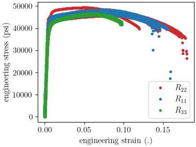
tension_fig = plt.figure(figsize=figsize, constrained_layout=True)
tension_data_collection.plot("engineering_strain", "engineering_stress",
                             state="temperature_5.330700e+02_direction_R22",
                             show=False, labels="$R_{22}$", figure=tension_fig,
                             color='tab:red')
tension_data_collection.plot("engineering_strain", "engineering_stress",
                             state="temperature_5.330700e+02_direction_R11",
                             show=False, labels="$R_{11}$", figure=tension_fig,
                             color='tab:blue')
tension_data_collection.plot("engineering_strain", "engineering_stress",
                             state="temperature_5.330700e+02_direction_R33",
                             labels="$R_{33}$", figure=tension_fig,
                             color='tab:green')
plt.xlabel("engineering strain (.)")
plt.ylabel("engineering stress (psi)")

tension_data_collection.remove_field("time")

top_hat_fig = plt.figure(figsize=figsize, constrained_layout=True)
top_hat_data_collection.plot("displacement", "load", show=False,
                             state="direction_R12", labels="$R_{12}$",
                             figure=top_hat_fig, color='tab:cyan')
top_hat_data_collection.plot("displacement", "load", show=False,
                             state="direction_R23", labels="$R_{23}$",
                             figure=top_hat_fig, color='tab:orange')
top_hat_data_collection.plot("displacement", "load",
                             state="direction_R31", labels="$R_{31}$",
                             figure=top_hat_fig, color='tab:purple')
plt.xlabel("displacement (in)")
plt.ylabel("displacement (lbs)")
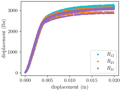
Text(20.771400166044003, 0.5, 'displacement (lbs)')
With the data prepared, we move on to building the models. The first step is to prepare the material model input deck file that is required by SIERRA/SM. We do this within python because the file is relatively short and simple. It also makes it easy to ensure naming is consistent in the SIERRA/SM input deck files and our MatCal objects. We create a string with the material model syntax that SIERRA/SM expects and the Aprepro variables that MatCal will populate with study and state parameters when running a study.
material_name = "6061T6_anisotropic_yield"
material_string = f"""
  begin material {material_name}
    density = 0.00026
    begin parameters for model hill_plasticity
      youngs modulus                = 10e6
      poissons ratio                = 0.33
      yield stress                  = {{yield_stress*1e3}}

      hardening model = voce
      hardening modulus = {{hardening*1e3}}
      exponential coefficient = {{b}}

      r11                           =   1
      r22                           =   {{R22}}
      r33                           =   {{R33}}
      r12                           =   {{R12}}
      r23                           =   {{R23}}
      r31                           =   {{R31}}
      coordinate system             =   rectangular_coordinate_system

      {{if(direction=="R11")}}
      direction for rotation        = 3
      alpha                         = 90.0
      {{elseif((direction=="R33") || (direction=="R31"))}}
      direction for rotation        = 1
      alpha                         = -90.0
      {{elseif(direction=="R23")}}
      direction for rotation        = 2
      alpha                         = 90.0
      {{endif}}
    end
  end
"""
We save that string to a file, so MatCal can add it to the model files that we generate for the tension and top hat shear test models.
material_filename = "hill_plasticity.inc"
with open(material_filename, 'w') as fn:
    fn.write(material_string)
MatCal communicates all required material
model information to its MatCal generated
finite element models through a Material
object, so we create the required object.
material = Material(material_name, material_filename, "hill_plasticity")
Now we create our tension model which requires the specimen geometry and model discretization options. We create a dictionary with all the required key words for creating the tension model mesh.
tension_geo_params = {"extensometer_length": 1.0,
            "gauge_length": 1.25,
            "gauge_radius": 0.125,
            "grip_radius": 0.25,
            "total_length": 4,
            "fillet_radius": 0.188,
            "taper": 0.0015,
            "necking_region":0.375,
            "element_size": 0.0125,
            "mesh_method":3,
            "grip_contact_length":1}
Then we create a RoundUniaxialTensionModel
that takes the material and geometry as input.
ASTME8_tension_model = RoundUniaxialTensionModel(material, **tension_geo_params)
A name is specified so that results information can be easily accessed and associated with this model. MatCal will generate a name for the model, but it may be convenient to supply your own.
ASTME8_tension_model.set_name('tension_specimen')
To ensure the model does not run longer than required for our
calibration, we use the
set_allowable_load_drop_factor()
method.
This will end the simulation when the load in the simulation
has decreased by 25% from peak load.
ASTME8_tension_model.set_allowable_load_drop_factor(0.25)
To complete the model, MatCal needs boundary condition information so that the model is deformed appropriately for each data set that is of interest to the calibration. We pass the uniaxial tension data collection to the model, so that it can form the correct boundary conditions for each state.
ASTME8_tension_model.add_boundary_condition_data(tension_data_collection)
Next, we set optional platform options. Since we will run this calibration on either an HPC cluster or a local machine, we setup the model with the appropriate platform specific options.
if is_sandia_cluster():
    ASTME8_tension_model.run_in_queue(MATCAL_WCID, 0.25)
    ASTME8_tension_model.continue_when_simulation_fails()
    platform = get_sandia_computing_platform()
    num_cores = platform.get_processors_per_node()
else:
    num_cores = 8
ASTME8_tension_model.set_number_of_cores(num_cores)
The model for the top hat shear test is built next. The same inputs are required for this model. First, we build a dictionary with all the needed geometry and discretization parameters.
top_hat_geo_params = {"total_height":1.25,
        "base_height":0.75,
        "trapezoid_angle": 10.0,
        "top_width": 0.417*2,
        "base_width": 1.625,
        "base_bottom_height": (0.75-0.425),
        "thickness":0.375,
        "external_radius": 0.05,
        "internal_radius": 0.05,
        "hole_height": 0.3,
        "lower_radius_center_width":0.390*2,
        "localization_region_scale":0.0,
        "element_size":0.005,
        "numsplits":1}
Next, we create the TopHatShearModel
and give it a name.
top_hat_model = TopHatShearModel(material, **top_hat_geo_params)
top_hat_model.set_name('top_hat_shear')
We set its allowable load drop factor and provide boundary condition data.
top_hat_model.set_allowable_load_drop_factor(0.05)
top_hat_model.add_boundary_condition_data(top_hat_data_collection)
Lastly, we setup the platform information for running the model.
top_hat_model.set_number_of_cores(num_cores*2)
if is_sandia_cluster():
  top_hat_model.run_in_queue(MATCAL_WCID, 30.0/60)
  top_hat_model.continue_when_simulation_fails()
We now create the objectives for the
calibration.
Both models are compared to the data
using a CurveBasedInterpolatedObjective.
The tension specimen is calibrated to the engineering stress/strain data
and the top hat specimen is calibrated to the load-displacement data.
tension_objective = CurveBasedInterpolatedObjective("engineering_strain", "engineering_stress")
top_hat_objective = CurveBasedInterpolatedObjective("displacement", "load")
With the objectives ready,
we create UserFunctionWeighting
objects that will remove data points from the data sets
that we do not want included in the calibration objective.
For the tension data, we remove the data in the elastic regime
and data near failure.
The following function does this by setting the residuals
that correspond to these features in the data to zero.
def remove_failure_points_from_residual(eng_strains, eng_stresses, residuals):
    import numpy as np
    weights = np.ones(len(residuals))
    peak_index = np.argmax(eng_stresses)
    peak_strain = eng_strains[peak_index]
    peak_stress = eng_stresses[peak_index]
    weights[(eng_strains > peak_strain) & (eng_stresses < 0.89*peak_stress)  ] = 0
    weights[(eng_strains < 0.005) ] = 0
    return weights*residuals
The preceding function is used to create
the UserFunctionWeighting object
for the tension objective and then added to the
objective as a weight.
tension_residual_weights = UserFunctionWeighting("engineering_strain",
                                                 "engineering_stress",
                                                 remove_failure_points_from_residual)
tension_objective.set_field_weights(tension_residual_weights)
A similar modification is required for the top hat data. Since the data in the failure region has been removed from the data itself, we only remove the data in the elastic region with the following function.
def remove_elastic_region_from_top_hat(displacements, loads, residuals):
    import numpy as np
    weights = np.ones(len(residuals))
    weights[(displacements < 0.005) ] = 0
    return weights*residuals
Then we create our
UserFunctionWeighting object
and apply it to the top hat objective.
top_hat_residual_weights = UserFunctionWeighting("displacement", "load",
                                                 remove_elastic_region_from_top_hat)
top_hat_objective.set_field_weights(top_hat_residual_weights)
Now we create the study parameters that will be calibrated. We provide reasonable bounds and assign their current value to be the initial point that we determined in 6061T6 aluminum anisotropy calibration initial point estimation.
yield_stress = Parameter("yield_stress", 15, 50, 42)
hardening = Parameter("hardening", 0, 60, 10.1)
b = Parameter("b", 10, 40, 35.5)
R22 = Parameter("R22", 0.8, 1.15, 1.05)
R33 = Parameter("R33", 0.8, 1.15, 0.95)
R12 = Parameter("R12", 0.8, 1.15, 1.0)
R23 = Parameter("R23", 0.8, 1.15, 0.97)
R31 = Parameter("R31", 0.8, 1.15, 0.94)
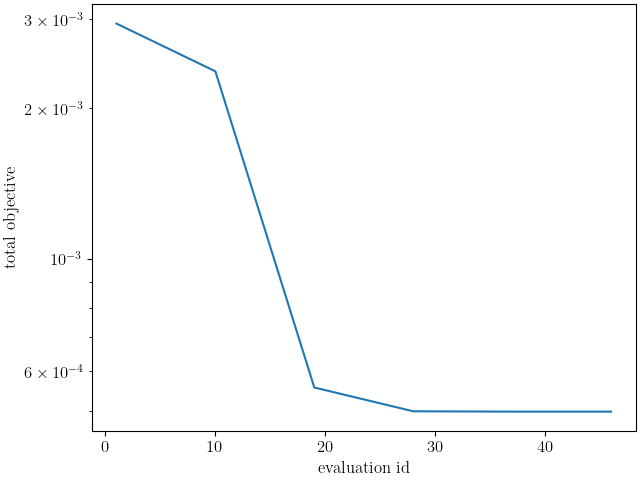
Finally, we can create our study. For
This calibration we use a
GradientCalibrationStudy.
study = GradientCalibrationStudy(yield_stress, hardening, b, R22, R33, R12, R23, R31)
study.set_results_storage_options(results_save_frequency=9)
We run the study in a subdirectory named 6061T6_anisotropy
to keep the current directory cleaner.
study.set_working_directory("6061T6_anisotropy", remove_existing=True)
We set the core limit so that it runs all model concurrently. MatCal knows if the models will be run in a queue on a remote node and will only assign one core to each model that is run in a queue. Since there are two models with three states and eight parameters we need to run a maximum of 54 concurrent models. On a cluster, we ensure that we can run all concurrently. On a local platform, we allow MatCal to use all processors that are available.
if is_sandia_cluster():
  study.set_core_limit(6*9+1)
else:
  study.set_core_limit(60)
We add evaluation sets for each model and data set and set the output verbosity to the desired level.
study.add_evaluation_set(ASTME8_tension_model, tension_objective, tension_data_collection)
study.add_evaluation_set(top_hat_model, top_hat_objective, top_hat_data_collection)
study.set_output_verbosity("normal")
The study is then launched and the best fit parameters will be printed and written to a file after it finished.
results = study.launch()
print(results.best.to_dict())
matcal_save("anisotropy_parameters.serialized", results.best.to_dict())
OrderedDict({'yield_stress': 43.468473637, 'hardening': 11.542110358, 'b': 12.38787657, 'R22': 1.0168744902, 'R33': 0.97813744911, 'R12': 0.96795492909, 'R23': 0.92103910221, 'R31': 0.91096757893})
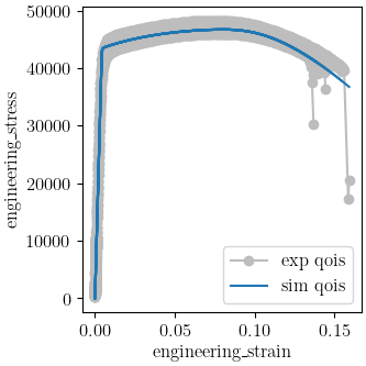
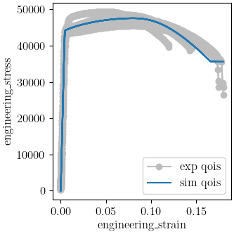
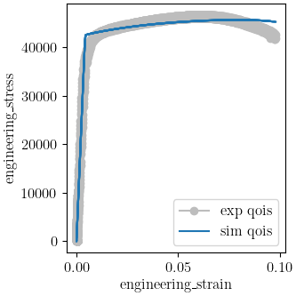
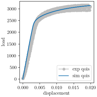
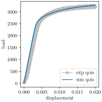
We use MatCal’s plotting features to plot the results and verify a satisfactory calibration has been achieved.
import os
init_dir = os.getcwd()
os.chdir("6061T6_anisotropy")
make_standard_plots("displacement", "engineering_strain")
os.chdir(init_dir)
Total running time of the script: (79 minutes 57.420 seconds)