Note

Go to the end to download the full example code.

304L stainless steel viscoplastic calibration

With our material model chosen and initial points determined, we can setup a final full finite element calibration to get a best fit to the available data.

Note

Useful Documentation links:

To begin, we import all the tools we will use. We will be using MatPlotLib, NumPy and MatCal.

import numpy as np
import matplotlib.pyplot as plt
from matcal import *
from site_matcal.sandia.computing_platforms import is_sandia_cluster, get_sandia_computing_platform
from site_matcal.sandia.tests.utilities import MATCAL_WCID

plt.rc('text', usetex=True)
plt.rc('font', family='serif')
plt.rc('font', size=12)
figsize = (4,3)

Next, we import the data using a BatchDataImporter. Since we are using a rate dependent material model, we assign displacement rate and initial temperature state variables to the data using set_fixed_state_parameters()

tension_data = BatchDataImporter("ductile_failure_ASTME8_304L_data/*.dat",
                                    file_type="csv")
tension_data.set_fixed_state_parameters(displacement_rate=2e-4, temperature=530)
tension_data = tension_data.batch

We then manipulate the data to fit our needs and modeling choices. First, we scale the data from ksi to psi units. Then we remove the time field as this has consequences for the finite element model boundary conditions. See Uniaxial tension solid mechanics boundary conditions.

tension_data = scale_data_collection(tension_data, "engineering_stress", 1000)
tension_data.remove_field("time")

Note

Above we remove the “time” field from the data. We do this to avoid any added computational cost incurred by feeding the measured displacement-time curve into the models as the boundary condition. Although this sometimes can result in a better calibration for a rate-dependent material model, it usually results in a more costly model due to additional time steps required to resolve the more complex loading history. This additional cost can be somewhat reduced by smoothing the provided boundary condition data to remove any noise, but not necessary for this mesh convergence study. As shown in 304L calibrated round tension model - effect of different model options, modeling the as-measured boundary condition has little effect on the calibration objective for this problem, so we will use the ideal boundary condition for all further models. By removing the “time” field, the boundary conditions are applied linearly at the correct rate due to our specification of “displacement_rate” in the data fixed states when the data is imported.

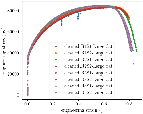
Next, we plot the data to verify we imported the data as expected.

astme8_fig = plt.figure(figsize=(5,4), constrained_layout=True)
tension_data.plot("engineering_strain", "engineering_stress",
                    figure=astme8_fig)
plt.xlabel("engineering strain ()")
plt.ylabel("engineering stress (psi)")

/gpfs/knkarls/projects/matcal_devel/external_matcal/matcal/core/data.py:588: UserWarning: Ignoring specified arguments in this call because figure with num: 1 already exists
  plt.figure(figure.number, constrained_layout=True)

Text(20.77140016604401, 0.5, 'engineering stress (psi)')

We also import the rate data as we will need to recalibrate the Johnson-Cook parameter $C$ since $Y_0$ will likely be changing. We put it in a DataCollection to facilitate plotting.

rate_data_collection = matcal_load("rate_data.joblib")

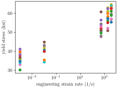
Next, we plot the data on with a semilogx plot to verify it imported as expected.

plt.figure(figsize=(4,3), constrained_layout=True)
def make_single_plot(data_collection, state, cur_idx, label,
                     color, marker, **kwargs):
    data = data_collection[state][cur_idx]
    plt.semilogx(state["rate"], data["yield"][0],
                marker=marker, label=label, color=color,
                **kwargs)

def plot_dc_by_state(data_collection, label=None, color=None,
                     marker='o', best_index=None, only_label_first=False, **kwargs):
    for state in data_collection:
        if best_index is None:
            for idx, data in enumerate(data_collection[state]):
                make_single_plot(data_collection, state, idx, label,
                                 color, marker, **kwargs)
                if ((color is not None and label is not None) or
                    only_label_first):
                    label = None
        else:
            make_single_plot(data_collection, state, best_index, label,
                             color, marker, **kwargs)
    plt.xlabel("engineering strain rate (1/s)")
    plt.ylabel("yield stress (ksi)")
plot_dc_by_state(rate_data_collection)

Based on the previous examples, we choose a material model with the following flow rule:

$\sigma_f=Y_0\left(\theta\right)\left[1+C\ln\left(\frac{\dot{\epsilon}^p} {\dot{\epsilon}_0}\right)\right] + A\left[1-\exp\left(-b\epsilon_p\right)\right]$

where $Y_0\left(\theta\right)$ is the temperature dependent, rate independent yield of the material, $\epsilon^p$ is the equivalent plastic strain, $C$ is a fitting parameter for the Johnson-Cook rate dependence of yield, and $A$ and $b$ are Voce hardening model parameters. For our yield surface, we will use the von Mises yield criterion. We calibrate this model with the following assumptions:

The elastic parameters and density can be used from [1] and will not be calibrated.
The temperature-dependence of $Y_0$ can be used from [1] and will not be calibrated.
The thermal properties (specific heat and thermal conductivity) can be taken from [29] while the conversion of plastic work to heat (the Taylor-Quinney coefficient) can be assumed to be 0.95.
The rate dependence parameters $Y_0$ and $C$ can be calibrated using a PythonModel and the 0.2% offset yield stress values extracted from the nonstandard tension data taken at several rates. Note that since the 0.2% offset yield measured in the experiments does not necessarily correspond to the material model $Y_0$ , the python model will have an additional parameter, $X$ , to compensate for this difference.
The remaining plasticity parameters $A$ and $b$ along with $Y_0$ can be calibrated using a RoundUniaxialTensionModel and the provided ASTME8 uniaxial tension data.

With these assumptions, we will begin by defining the MatCal Parameter objects for the calibration. These require the parameter name which will be passed into the models, parameter bounds and the parameter current value. For this calibration the parameter bounds were based on previous experience with the model and inspection of the data. The initial values come from 304L bar data analysis and 304L bar calibration initial point estimation. First, we read in the results from those examples and then create the parameters with the appropriate initial points.

voce_params = matcal_load("voce_initial_point.serialized")
jc_params = matcal_load("JC_parameters.serialized")

Y_0 = Parameter("Y_0", 20, 60,
                voce_params["Y_0"])
A = Parameter("A", 100, 400,
              voce_params["A"])
b = Parameter("b", 0, 3,
              voce_params["b"])
C = Parameter("C", -3, -1,
              np.log10(jc_params["C"]))
X = Parameter("X", 0.50, 1.75, 1.0)

Now we can define the models to be calibrated. We will start with the Python function for the rate-dependence Python model.

def JC_rate_dependence_model(Y_0, A, b, C, X, ref_strain_rate, rate,  **kwargs):
    yield_stresses = np.atleast_1d(Y_0*X*(1+10**C*np.log(rate/ref_strain_rate)))
    yield_stresses[np.atleast_1d(rate) < ref_strain_rate] = Y_0
    return {"yield":yield_stresses}

We then create the model and add the reference strain rate constant to the model.

rate_model = PythonModel(JC_rate_dependence_model)
rate_model.set_name("python_rate_model")
rate_model.add_constants(ref_strain_rate=1e-5)

In the JC_rate_dependence_model function, you can see that the correction factor $X$ is a simple multiplier on $Y_0$ . This allows the calibration algorithm to compensate for any discrepancy between the 0.2% offset yield in the experimental measurements and the material model yield. The correction factor is not actually used in the SIERRA/SM material model.

With the rate model defined, we can now build the MatCal standard model for the ASTME8 tension specimen. MatCal’s RoundUniaxialTensionModel does not enforce the requirements of the ASTME8 test specification, and will build the model according to the geometry and input provided. It significantly simplifies generating a model of the test for calibration. The primary inputs to create the model are: the geometry for the specimen, a material model input file, and data for boundary condition generation. For more details on the model and its features see MatCal Generated SIERRA Standard Models and Uniaxial Tension Models.

First, we create the Material object. We write the material file that will be used to create the MatCal Material.

material_name = "304L_viscoplastic"
with open("yield_temp_dependence.inc", 'r') as f:
    temp_dependence_func = f.read()

material_string = f"""
    begin definition for function 304L_yield_temp_dependence
        #loose linear estimate of data from MMPDS10 Figure 6.2.1.1.4a
        type is piecewise linear
        begin values
        {temp_dependence_func}
        end
    end

    begin definition for function 304_elastic_mod_temp_dependence
        #Stender et. al.
        type is piecewise linear
        begin values
            294.11,     1
            1673,      0.4
        end
    end

    begin definition for function 304L_thermal_strain_temp_dependence
        #Stender et. al.
        type is piecewise linear
        begin values
            294.11, 0.0
            1725.0, 0.02
        end
    end

    begin material {material_name}
        #density and elastic parameters from Granta's MMPDS10 304L database Table 2.7.1.0(b3).
        #Design Mechanical and Physical Properties of AISI 304 Stainless Steels

        density = {{density}}
        thermal engineering strain function = 304L_thermal_strain_temp_dependence

        begin parameters for model j2_plasticity
            youngs modulus                = 29e6
            poissons ratio                =   0.27
            yield stress                  = {{Y_0*1e3}}

            youngs modulus function = 304_elastic_mod_temp_dependence

            hardening model = decoupled_flow_stress

            isotropic hardening model = voce
            hardening modulus = {{A*1e3}}
             exponential coefficient = {{b}}

            yield rate multiplier = johnson_cook
            yield rate constant = {{10^C}}
            yield reference rate = {{ref_strain_rate}}


            yield temperature multiplier = user_defined
            yield temperature multiplier function = 304L_yield_temp_dependence

            hardening rate multiplier = rate_independent
            hardening temperature multiplier = temperature_independent

            thermal softening model      = coupled
            beta_tq                      = 0.95
            specific heat = {{specific_heat}}
        end
    end
"""

The study parameters and other parameters can be seen in the file and are identified with the curly bracket identifiers for Aprepro [28] substitution when the study is running. Also, the functions needed in the model for temperature dependence are included.

Note

For this material model, the material file for SIERRA/SM also contains the density and specific heat variables that are needed for coupled simulations. We have included them here so that we can investigate coupling in a follow-on study. If you want these to be added by MatCal, they can be added to the material model input using curly bracket identifiers as shown above. MatCal will substitute the appropriate values into the file if they are to the model as MatCal SIERRA model constants, MatCal state parameters, MatCal study parameters or if they are added using the activate_thermal_coupling() method. Alternatively, they can be entered manually as fixed values. If they are entered as shown above and MatCal does not substitute values for their identifiers, they will default to zero which could cause errors depending on the model options chosen.

Next, we save the material string to a file, so MatCal can add it to the model files that we generate for the tension model. We then create the MatCal Material object.

material_filename = "304L_viscoplastic_voce_hardening.inc"
with open(material_filename, 'w') as fn:
    fn.write(material_string)

sierra_material = Material(material_name, material_filename,
                            "j2_plasticity")

Next, we create the tension model using the RoundUniaxialTensionModel which takes the material object we created and geometry parameters as input. It is convenient to put the geometry parameters in a dictionary and then unpack that dictionary when initializing the model as shown below. After the model is initialized, the model’s options can be set and modified as desired. Here we pass the entire data collection into the model for boundary condition generation. Since our data collection no longer has the test displacement-time history, the model will deform the specimen to the maximum displacement in the data over the correct time to achieve the desired engineering strain rate. We study the effects of boundary condition choice in more detail in 304L calibrated round tension model - effect of different model options.

geo_params = {"extensometer_length": 0.75,
               "gauge_length": 1.25,
               "gauge_radius": 0.125,
               "grip_radius": 0.25,
               "total_length": 4,
               "fillet_radius": 0.188,
               "taper": 0.0015,
               "necking_region":0.375,
               "element_size": 0.01,
               "mesh_method":3,
               "grip_contact_length":1}

astme8_model = RoundUniaxialTensionModel(sierra_material, **geo_params)
astme8_model.add_boundary_condition_data(tension_data)

We set the cores the model uses to be platform dependent. On a local machine it will run on 36 cores. If its on a cluster, it will run in the queue on 112.

astme8_model.set_number_of_cores(24)
if is_sandia_cluster():
    astme8_model.run_in_queue(MATCAL_WCID, 0.5)
    astme8_model.continue_when_simulation_fails()
    platform = get_sandia_computing_platform()
    cores_per_node = platform.get_processors_per_node()
    astme8_model.set_number_of_cores(cores_per_node)
astme8_model.set_allowable_load_drop_factor(0.45)
astme8_model.set_name("ASTME8_tension_model")

We also add the reference strain rate constant to the SIERRA model.

astme8_model.add_constants(ref_strain_rate=1e-5)

After preparing the models and data, we must define the objectives to be minimized. For this calibration, we will need a separate objective for each model and data set to be compared. Both will use the CurveBasedInterpolatedObjective, but will differ in the fields that they use for interpolation and residual calculation. For the rate dependence model, we will be calibrating the yield stress from the model to each measured yield at each rate. For the tension model, we will be calibrating to the measured engineering stress-strain curve. Therefore, we create the objectives shown below.

rate_objective = Objective("yield")
astme8_objective = CurveBasedInterpolatedObjective("engineering_strain", "engineering_stress")

We then create a function and set of objects that will set certain values in the residual vector to zero based on values in the data curve used to calculate that residual vector. This is to remove residuals corresponding to portions of the curve that we should not calibrate to or do not wish to calibrate to.

def remove_uncalibrated_data_from_residual(engineering_strains, engineering_stresses, residuals):
    import numpy as np
    weights = np.ones(len(residuals))
    weights[engineering_stresses < 38e3] = 0
    weights[engineering_strains > 0.75] = 0
    return weights*residuals

residual_weights = UserFunctionWeighting("engineering_strain", "engineering_stress",
                                         remove_uncalibrated_data_from_residual)
astme8_objective.set_field_weights(residual_weights)

Note

Above we remove the elastic and steep unloading portions of the stress-strain curves from the objective using UserFunctionWeighting object. As stated previously, the elasticity constants are pulled from the literature, so keeping the elastic data in the objective is not needed. Additionally, the steep unloading after necking will not be well captured with a coarse mesh and the absence of a failure method such as element death. Refining the mesh and adding failure significantly increases the cost of the model with little effect on the calibration results. At a minimum, we need the calibration to be able to identify the peak load and strain at peak load in the data which for this data only requires strains up to 0.75. This step is not necessarily required, but it does reduce the computational cost of the calibration and most likely results in an improved calibration.

To perform the calibration, we will use the GradientCalibrationStudy. First, we create the calibration study object with the Parameter objects that we made earlier. We then add the evaluation sets which will be combined to form the full objective. In this case, each evaluation set has a single objective, model and data/data_collection. As a result, MatCal will track two objectives for this problem.

Note

MatCal can also accept multiple objectives passed to a single evaluation set in the form of an ObjectiveCollection. You can also add evaluation sets for a given model multiple times. This is useful when you have different types of data from the experiments and must use different objectives on these data sets. An example would be calibrating to both stress-strain and temperature-time data. Sometimes the experimental data is not collocated in time and supplied in different files. In such a case, you could calibrate to both by adding two evaluation sets for the model, one for stress-strain and another for temperature-time.

After adding the evaluation sets, we need to set the study core limit. MatCal takes advantage of multiple cores in two layers. Most models can be run on several cores, all studies can run evaluation sets in parallel (all models for a combined objective evaluation can be run concurrently), and most studies can run several combined objective evaluations concurrently. For this case, we need 1 core for the python model and 36 cores for the tension model in each combined objective evaluation. The study itself supports objective evaluation concurrently up to $n+1$ where $n$ is the number of parameters. See the study specific documentation for the objective evaluation concurrency for other methods. For this case, the study will perform six (five parameters + 1) concurrent combined objective evaluations, so this study can use at most 37*6 cores. Since this is a relatively large number of cores, we set the core limit to 112. This limit is total number of cores we can use on the computational resources we plan to run this on. If you have fewer cores, set the limit to what is available and MatCal will not use more than what is specified. If no core limit is set, MatCal will default to 1. For parallel jobs, you must specify the limit or MatCal will error out. These specifications are for running jobs on a local machine.

calibration = GradientCalibrationStudy(Y_0, A, b, C, X)
calibration.add_evaluation_set(astme8_model, astme8_objective, tension_data)
calibration.set_results_storage_options(results_save_frequency=6)
calibration.add_evaluation_set(rate_model, rate_objective, rate_data_collection)
calibration.set_core_limit(112)
cal_dir = "finite_element_model_calibration"
calibration.set_working_directory(cal_dir, remove_existing=True)

However, if we are on a cluster where the models are run in a queue (not the local machine), we set the limit based on the number of jobs that can run concurrently because there is some overhead for job monitoring and results processing. For our case, that is only six python models run on the parent node and then six finite element models run on children nodes with job monitoring and post processing on the parent node.

if is_sandia_cluster():
    calibration.set_core_limit(12)

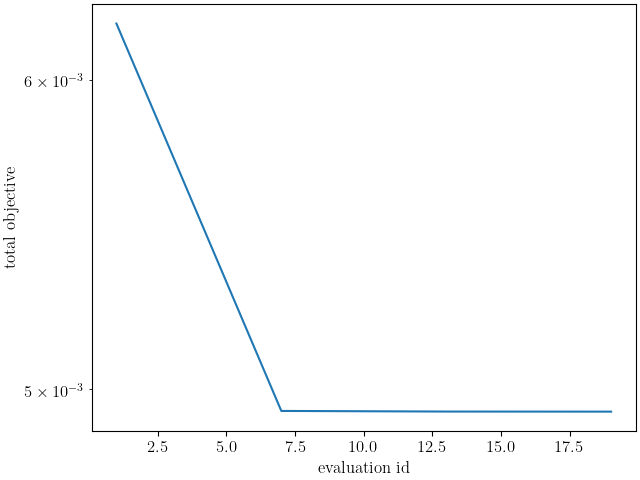
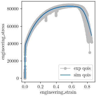
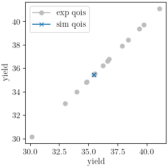
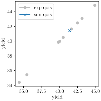
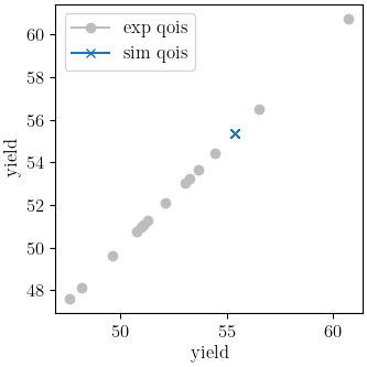
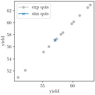
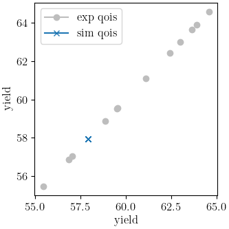
We can now run the calibration. After it finishes, we will plot MatCal’s standard plots which include plotting the simulation QoIs versus the experimental data QoIs, the objectives versus evaluation and the objectives versus the parameter values. We also print and save the final parameter values.

results = calibration.launch()
print(results.best)
matcal_save("voce_calibration_results.serialized", results.best.to_dict())
import os
init_dir = os.getcwd()
os.chdir(cal_dir)
make_standard_plots("engineering_strain","yield")
os.chdir(init_dir)

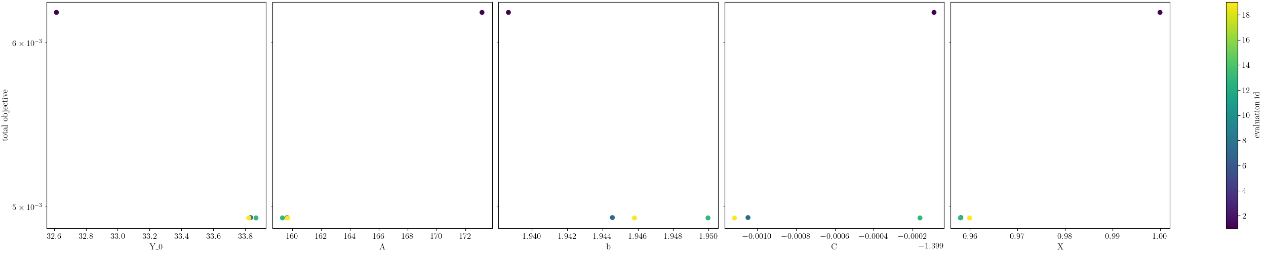
Y_0: 33.822903791
A: 159.67098523
b: 1.9458059132
C: -1.4001161716
X: 0.95998543176

The calibration finishes successfully with the Dakota output:

**** RELATIVE FUNCTION CONVERGENCE *****

indicating that the calibration completed successfully. The QoI plots also show that the calibration matches the data well. The objective results for the best evaluation are given in the output shown below.:

Evaluation results for "matcal_workdir.25":
        Objective "CurveBasedInterpolatedObjective_1" for model "ASTME8_tension_model" = 0.00028227584006352657
        Objective "CurveBasedInterpolatedObjective_0" for model "python_rate_model" = 0.0033173052116014117

The tension model objective is fairly low while the python rate model objective is noticeably higher. These objectives will never be zero due to the fact that there is model form error that is unavoidable and due to the variance in the data. From the QoI plots it is clear that the rate data have noticeably higher variability for the measured dependent field (“yield”) at a given independent field value (“rate”) when compared to the tension engineering stress-strain data. This is likely the primary cause for its higher objective value. This demonstrates why it is typically a good practice to weight objectives or residuals by the inverse of the variance or noise of the data. MatCal will do this if the data variance is provided with the data and the user adds NoiseWeightingFromFile residuals weights to the objective with set_field_weights(). The same can be accomplished by the user by using the ConstantFactorWeighting with the appropriate scale factor. For this problem, the calibration is acceptable without it and it is not necessarily needed because objectives are fairly decoupled. However, using this weighting would result in a small change to the calibrated parameters if used.

Total running time of the script: (17 minutes 34.189 seconds)

Gallery generated by Sphinx-Gallery