Sparse Grid Adaptive Surrogate Example

This example demonstrates how to generate a surrogate using a MatCal study that performs adaptive sampling for training the surrogate. This study is a follow-on example to Surrogate Generation Example and uses the same boundary value problem that from example. The primary difference is that a Matcal adaptive surrogate study is used for surrogate training. In this example we use a SparseGridAdaptiveSurrogateStudy to create the surrogate.

We re-create the model and parameters from Surrogate Generation Example that are needed to perform the study.

# sphinx_gallery_thumbnail_number = 2
import matcal as mc
import numpy as np

conv_heat_transfer_coeff = mc.Parameter("H", 1, 100) # W / (m^2 K)
far_field_temperature = mc.Parameter("T_inf", 500, 1000) # K
air_temperature = mc.Parameter("T_air", 400, 800) # K

my_hifi_model = mc.UserDefinedSierraModel('aria', "aria_model/metal_foam_layers.i",
                                          "aria_model/test_block.g", "aria_model/include")
my_hifi_model.set_results_filename("results/results.csv")
my_hifi_model.set_number_of_cores(2)
from site_matcal.sandia.tests.utilities import MATCAL_WCID
from site_matcal.sandia.computing_platforms import is_sandia_cluster

if is_sandia_cluster():
    my_hifi_model.run_in_queue(MATCAL_WCID, 0.25)
    my_hifi_model.continue_when_simulation_fails()
    my_hifi_model.set_number_of_cores(12)

With the model and parameters created, we must still define the independent variable for the surrogate and the values at which we want the surrogate to produce a response. However, we do not create the objective. This will automatically happen inside the study. This is done because only one response can be used to build the surrogate for because the adaptive training technique uses the sensitivity of the response to the input parameters to adaptively choose where to add training samples.

n_prediction_points = 200
time_start = 0
time_end = 60 * 60 * 2
indep_field_vals = np.linspace(time_start, time_end, n_prediction_points)

We can now create the study. As stated previously, only one response can be reproduced with an adaptive surrogate study. As a result, the study requires the specification of the independent field, the values for the independent field, and the target field for which the surrogate will predict the response. For this study, we choose the bottom thermocouple response as the target field because it had the highest error for both of the test cases from the non-adaptive surrogate example.

study = mc.SparseGridAdaptiveSurrogateStudy(conv_heat_transfer_coeff, far_field_temperature,
                                        air_temperature)
study.set_independent_variable("time", indep_field_vals)
study.set_target_field_name("TC_bottom")
study.add_evaluation_set(my_hifi_model)

We must also specify how many samples to run for generating test data. These adaptive surrogates use Halton sampling for test data generation.

study.set_number_of_test_samples(50)

Next we set a stopping criteria. We are hoping to increase the accuracy of the surrogate to be within 1.5 K or less for all time for all test cases. We do so with the set_error_stopping_criteria() that sets a stopping criteria based on the test sample error.

study.set_error_stopping_criteria(max_abs_error_goal=1.5)

Now, we set the max number of training samples to the same number of samples that were used for the non-adaptive surrogate. In theory, adaptivity should improve the prediction with the same or fewer samples.

study.set_max_training_samples(500)

Finally, we set the surrogate save filename and basic study options.

study.set_surrogate_save_filename("layered_metal_bc_SG_adaptive_surrogate.joblib")
if is_sandia_cluster():
    study.set_core_limit(250)
else:
    study.set_core_limit(112)

If setting the seed, ensure the test group seed is different than the study seed. If not, the training data will include samples from the test data.

study.set_test_group_random_seed(12345)
study.set_seed(54321)
study.set_working_directory("sparse_grid_surrogate", remove_existing=True)

With our study defined, we run it and wait for it to complete.

study_results = study.launch()

We can now access our surrogate using the surrogate() property. The surrogate is a SparseGridAdaptiveSurrogate object.

surrogate = study.surrogate

The study_results variable is a StudyResults object with the training results store in it.

While the surrogate is being trained, the generator will report the testing score for the target response the surrogate was requested to predict. Like with the non-adaptive surrogate, the best score for any test is 1, with poorer scores less than 1. The test score indicates how well the surrogate performs on data it was not trained on. Currently, training scores are not reported for the SparseGridAdaptiveSurrogateStudy. The score is output in the log files and standard output, but can also be accessed through a method under the surrogate after it has been produced. We print the score below for this surrogate.

print('Test scores:\n', surrogate.score())

Test scores:
 0.9899359687882371

Both the test scores and the training scores indicate the surrogate is well trained and can be used to predict our response.

Now we use the surrogate to make predictions of the model responses. The order of the parameters is the same order that they were passed into the the parameter collection or study, but this can be verified by calling parameter_order(). By default, the surrogates will not allow evaluations outside of the parameter space ranges provided in the parameter bounds passed to the adaptive surrogate study used for training.

We evaluate the surrogate and resulting error similar to as was done in the previous non-adaptive surrogate example so that we can see if the surrogate has a more accurate prediction.

H = 10
T_inf = 600
T_air = 500

H2 = 20
T_inf2 = 815
T_air2 = 634

prediction = surrogate([[H, T_inf, T_air], [H2, T_inf2, T_air2]], batch_evaluate=True)

param_study = mc.ParameterStudy(conv_heat_transfer_coeff, far_field_temperature,
                                 air_temperature)
my_objective = mc.SimulationResultsSynchronizer('time', indep_field_vals,
                                                 "TC_top", "TC_bottom")
param_study.add_evaluation_set(my_hifi_model, my_objective)
param_study.set_core_limit(16)
param_study.add_parameter_evaluation(H=H, T_inf=T_inf, T_air=T_air)
param_study.add_parameter_evaluation(H=H2, T_inf=T_inf2, T_air=T_air2)
results = param_study.launch()

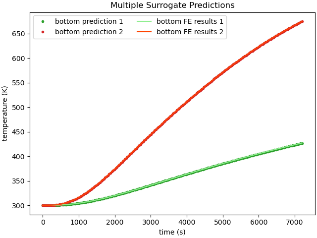
With both the finite element model results and the surrogate model results obtained, we can plot them together for comparison. Note that we can only plot the bottom thermocouple because adaptive surrogates are specific for a given response.

fe_data1 = results.simulation_history[my_hifi_model.name]["matcal_default_state"][0]
fe_data2 = results.simulation_history[my_hifi_model.name]["matcal_default_state"][1]

import matplotlib.pyplot as plt
plt.close('all')
plt.figure(constrained_layout=True)
plt.plot(prediction['time'], prediction['TC_bottom'][0,:], '.', label="bottom prediction 1",
         color='tab:green')
plt.plot(prediction['time'], prediction['TC_bottom'][1,:], '.', label="bottom prediction 2",
         color='tab:red')

plt.plot(fe_data1['time'], fe_data1['TC_bottom'], label="bottom FE results 1",
         color='lightgreen')
plt.plot(fe_data2['time'], fe_data2['TC_bottom'], label="bottom FE results 2",
         color='orangered')
plt.xlabel("time (s)")
plt.ylabel("temperature (K)")

plt.legend(ncols=2)
plt.title("Multiple Surrogate Predictions")

plt.show()

Similarly, we can plot the surrogate model error. First, we interpolate the surrogate results to the finite element model times. Next, we calculate and plot the absolute error for each prediction.

interp_prediction_bot1 = np.interp(fe_data1['time'], prediction['time'],
                                     prediction['TC_bottom'][0,:])
interp_prediction_bot2 = np.interp(fe_data2['time'], prediction['time'],
                                     prediction['TC_bottom'][1,:])

plt.figure(constrained_layout=True)
plt.plot(fe_data1['time'], interp_prediction_bot1-fe_data1['TC_bottom'],
         label="bottom TC error 1",
         color='tab:green')
plt.plot(fe_data2['time'], interp_prediction_bot2-fe_data2['TC_bottom'],
         label="bottom TC error 2",
         color='tab:red')
plt.xlabel("time (s)")
plt.ylabel("temperature error (K)")

plt.legend(ncols=2)
plt.title("Multiple Surrogate Predictions")

plt.show()

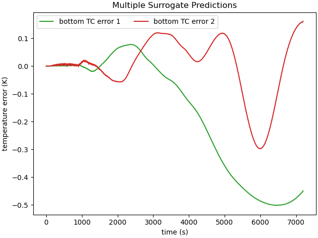
The sparse grid surrogate shows much reduced error for the chosen samples points when compared to the non-adaptive surrogate from Surrogate Generation Example. For these two samples, The error is less than 1 K for all time. However, the adaptive surrogate did not reach this low value for all 50 samples in the test set. However, it did reach the convergence criteria of a maximum error for all test samples of 1.5 K at 353 samples. You can access this information using the max_error_history() and sample_count_history() properties.

print("Max error:", surrogate.max_error_history[-1])
print("Training samples:", surrogate.sample_count_history[-1])

Max error: 1.4860231166993572
Training samples: 353

Since adaptive surrogates in MatCal also save the training error history, we can plot the error metrics for the surrogate as a function of model training samples used. This can useful to evaluate convergence rate and to assess if better performance is likely with additional training samples.

plt.figure(constrained_layout=True)
plt.plot(surrogate.sample_count_history, surrogate.max_error_history,'o',
         color='tab:red')
plt.xlabel("training samples")
plt.ylabel("max test sample error (K)")
plt.title("Surrogate error convergence")
plt.show()

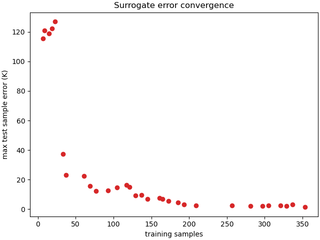
We can see in the convergence plot, that the error has stagnated. More iterations will likely not improve the performance of the surrogate.