Full-field Interpolation Calibration Verification

This example is a repeat of the Load Displacement Calibration Verification - First Attempt with the addition of a full-field interpolating objective.

There are only two differences between this calibration and the load-displacement calibration.

1. We add full-field displacement data to the calibration. We use the InterpolatedFullFieldObjective for this comparison where the fields compared are the X and Y displacements. We do this comparison at four points in the load displacement history: (1) near yield, (2) approximately halfway through the total displacement, (3) at peak load and (4) at 92.5% of peak load past peak load.

2. We also change the extrapolation values in the load-displacement CurveBasedInterpolatedObjective to be four times the max load of the synthetic data in an attempt to avoid local objectives in the load-displacement objective when the curves cross.

All other inputs remain the same. As a result, the commentary is mostly removed for this example except for some discussion on the results at the end.

from matcal import *
import numpy as np

synthetic_data = FieldSeriesData("../../../docs_support_files/synthetic_surf_results_0_degree.e")
synthetic_data.rename_field("U", "displacement_x")
synthetic_data.rename_field("V", "displacement_y")
synthetic_data.rename_field("W", "displacement_z")

peak_load_arg = np.argmax(synthetic_data["load"])
last_desired_arg = np.argmin(np.abs(synthetic_data["load"]\
                                    [peak_load_arg:]-np.max(synthetic_data["load"])*0.925))
synthetic_data = synthetic_data[:last_desired_arg+1+peak_load_arg]

last_disp_arg = np.argmax(synthetic_data["displacement"])
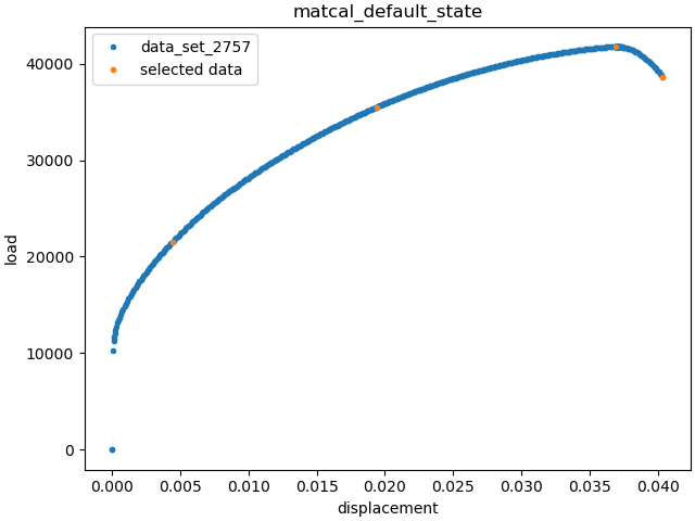
selected_data = synthetic_data[[50, 200, peak_load_arg, last_disp_arg]]
selected_data.set_name("selected data")

dc = DataCollection("synthetic", synthetic_data, selected_data)
dc.plot("displacement", "load")

import matplotlib.pyplot as plt
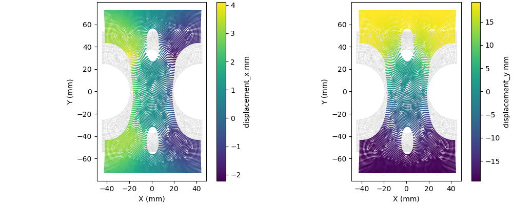
def plot_field(data, field, ax):
    c = ax.scatter(1e3*(data.spatial_coords[:,0]),
                   1e3*(data.spatial_coords[:,1]),
                   c="#bdbdbd", marker='.', s=1, alpha=0.5)
    c = ax.scatter(1e3*(data.spatial_coords[:,0]+data["displacement_x"][-1, :]),
                   1e3*(data.spatial_coords[:,1]+data["displacement_y"][-1, :]),
                   c=1e3*data[field][-1, :], marker='.', s=3)
    ax.set_xlabel("X (mm)")
    ax.set_ylabel("Y (mm)")
    ax.set_aspect('equal')
    fig.colorbar(c, ax=ax, label=f"{field} mm")

fig, axes = plt.subplots(1,2, figsize=(10,4), constrained_layout=True)
plot_field(synthetic_data, "displacement_x", axes[0])
plot_field(synthetic_data, "displacement_y", axes[1])
plt.show()

mat_file_string = """begin material test_material
  density = 1
  begin parameters for model hill_plasticity
    youngs modulus  = {elastic_modulus*1e9}
    poissons ratio  = {poissons}
    yield_stress    = {yield_stress*1e6}

    hardening model = voce
    hardening modulus = {A*1e6}
    exponential coefficient = {n}

    coordinate system = rectangular_coordinate_system

    R11 = {R11}
    R22 = {R22}
    R33 = {R33}
    R12 = {R12}
    R23 = {R23}
    R31 = {R31}
  end
end
"""

with open("modular_plasticity.inc", 'w') as fn:
    fn.write(mat_file_string)


model = UserDefinedSierraModel("adagio", "synthetic_data_files/test_model_input_reduced_output.i",
                               "synthetic_data_files/test_mesh.g", "modular_plasticity.inc")
model.set_name("test_model")
model.add_constants(elastic_modulus=200, poissons=0.27, R22=1.0,
                    R33=0.9, R23=1.0, R31=1.0)
model.read_full_field_data("surf_results.e")
from site_matcal.sandia.computing_platforms import is_sandia_cluster, get_sandia_computing_platform
from site_matcal.sandia.tests.utilities import MATCAL_WCID

num_cores=96
if is_sandia_cluster():
    model.run_in_queue(MATCAL_WCID, 0.5)
    model.continue_when_simulation_fails()
    platform = get_sandia_computing_platform()
    num_cores = platform.get_processors_per_node()
model.set_number_of_cores(num_cores)

interpolate_objective = InterpolatedFullFieldObjective("synthetic_data_files/test_mesh_surf.g",
                                                       "displacement_x",
                                                       "displacement_y")
interpolate_objective.set_name("interpolate_objective")

max_load = float(np.max(synthetic_data["load"]))
load_objective = CurveBasedInterpolatedObjective("displacement", "load",
                                                 right=max_load*4)
load_objective.set_name("load_objective")

Y = Parameter("yield_stress", 100, 500.0, 218.0)
A = Parameter("A", 100, 4000, 1863.0)
n = Parameter("n", 1, 10, 1.28)
R11 = Parameter("R11", 0.8, 1.1)
R12 = Parameter("R12", 0.8, 1.1)

param_collection = ParameterCollection("Hill48 in-plane", Y, A, n, R11, R12)

study = GradientCalibrationStudy(param_collection)
study.set_results_storage_options(results_save_frequency=len(param_collection)+1)
study.set_core_limit(100)
study.add_evaluation_set(model, load_objective, synthetic_data)
study.add_evaluation_set(model, interpolate_objective, selected_data)
study.set_working_directory("ff_interp_cal_initial", remove_existing=True)
study.set_step_size(1e-4)
study.do_not_save_evaluation_cache()

results = study.launch()
calibrated_params = results.best.to_dict()
print(calibrated_params)

goal_results = {"yield_stress":200,
                "A":1500,
                "n":2,
                "R11":0.95,
                "R12":0.85}

def pe(result, goal):
    return (result-goal)/goal*100
for param in goal_results.keys():
    print(f"Parameter {param} error: {pe(calibrated_params[param], goal_results[param])}")

• 
• 

Opening exodus file: ../../../docs_support_files/synthetic_surf_results_0_degree.e
Opening exodus file: ../../../docs_support_files/synthetic_surf_results_0_degree.e
Closing exodus file: ../../../docs_support_files/synthetic_surf_results_0_degree.e
Closing exodus file: ../../../docs_support_files/synthetic_surf_results_0_degree.e
Opening exodus file: synthetic_data_files/test_mesh_surf.g
Closing exodus file: synthetic_data_files/test_mesh_surf.g
Opening exodus file: synthetic_data_files/test_mesh_surf.g
Closing exodus file: synthetic_data_files/test_mesh_surf.g
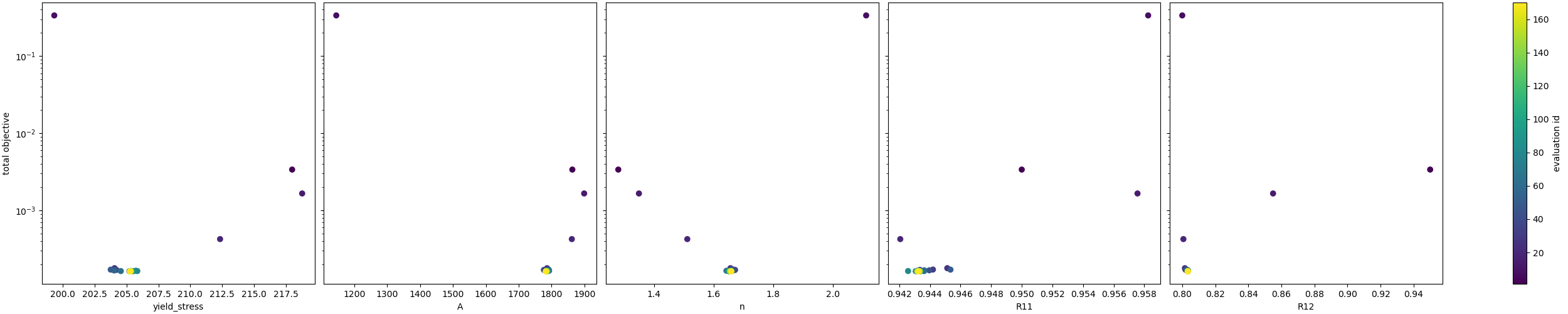
OrderedDict({'yield_stress': 205.26957029, 'A': 1782.5516248, 'n': 1.6587624642, 'R11': 0.94325998084, 'R12': 0.80333563582})
Parameter yield_stress error: 2.634785144999995
Parameter A error: 18.83677498666666
Parameter n error: -17.061876789999996
Parameter R11 error: -0.7094757010526315
Parameter R12 error: -5.489925197647056

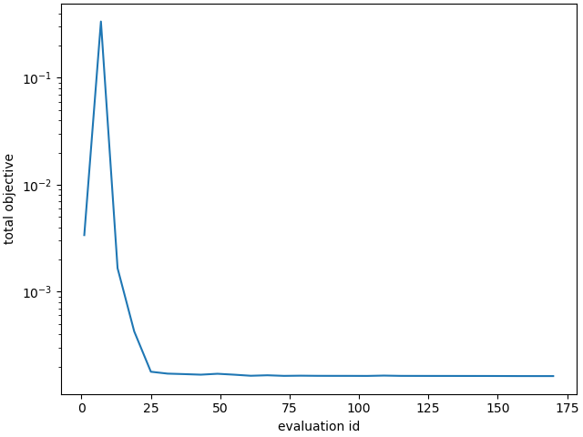
The calibrated parameter percent errors are much improved over the load-displacement curve only calibration. However, errors still exist that are larger than desired and the calibration completes with FALSE CONVERGENCE. A possible way to improve the calibration could be to add the 90_degree data set to the calibration.

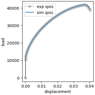
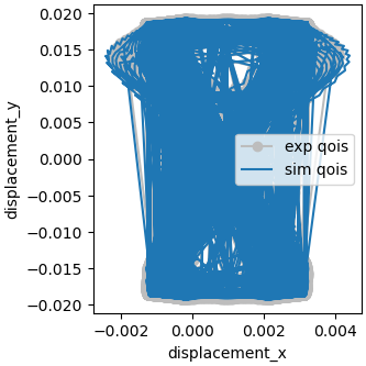
When we plot the results below, we see that the results for the load-displacement curve agree well with the synthetic data. The improvement is due to the algorithm driving the full-field interpolation objective down. This indicates that the full-field interpolation was the driver for the improvements gained with this calibration. Overall, adding the full-field data improved the calibration performance and the results are satisfactory for use in follow-on simulations even if not accurate enough for verification purposes.

Note

The QoIs are purposefully not plotted for the full-field interpolation objective. This is done to avoid saving and moving the large data sets which can exacerbated out-of-memory issues.

import os
init_dir = os.getcwd()
os.chdir("ff_interp_cal_initial")
make_standard_plots("displacement","displacement_x")
os.chdir(init_dir)
# sphinx_gallery_thumbnail_number = 5

• 
• 
• 
•