Polynomial HWD Verification with Colocated Points

In this example, we use an analytical function to test and verify our use and implementation of the Polynomial HWD algorithm where the points are colocated. The colocation is done using our PyCompadre’s GMLS algorithm [15]. We use the algorithm to map the experimental data onto the simulation points. Once this is done, the HWD method can be used to compare the data. We designed the verification problem to be representative of intended application and use full-field data that captures much of the expected behavior seen in real data sets. This test will compare the significant weights of the full-field data in their compressed latent space. Since the HWD modes are guaranteed to be the same, comparing the weights will be a valid comparison of the field as long as the field accurately reproduced with sufficient modes and as long as the GMLS interpolation doesn’t adversely affect the field.

Once again, we will generate two instances of our full-field data with noise and strive to have their difference be as small as possible. The same procedure is used here a was used in Polynomial HWD Verification - Analytical Function.

To begin we import the libraries and tools we will be using to perform this study.

from matcal import *
import numpy as np
import matplotlib.pyplot as plt

plt.rc('text', usetex=True)
plt.rc('font', family='serif')
plt.rcParams.update({'font.size': 12})

First, we defined the domain for our measured grid using NumPy tools. The domain is about 15 mm high (6 inches) and 7.6 mm wide (3 inches). The measured grid has 300 points in each dimension (x, y).

H = 6*0.0254
W = 3*0.0254

measured_num_points = 300
measured_xs = np.linspace(-W/2, W/2, measured_num_points)
measured_ys = np.linspace(-H/2, H/2, measured_num_points)

measured_x_grid, measured_y_grid = np.meshgrid(measured_xs, measured_ys)

Next, we will define our test function. We are interested in generating a function that is representative of the full-field data we will use in calibrations and other MatCal studies. Generally, these data will be smooth, have some lower frequency and higher frequency behavior and may have areas of localized high gradients and values. As a result we choose, the following function which is an additive combination of three sinusoids and a linear function that is multiplied by a smooth function that approximates a dirac. This function is defined below:

def analytical_function(X,Y):
    small = H/10
    func = (H/5 * np.sin(np.pi*Y/2/(H/2)) - W/50 * X/(W/2)
           + H/40*np.sin(np.pi*Y/2/(H/20)) + W/100*np.sin(X/(W/20))) \
           * (1+small/(np.pi*(X**2+Y**2+small**2)))
    return func

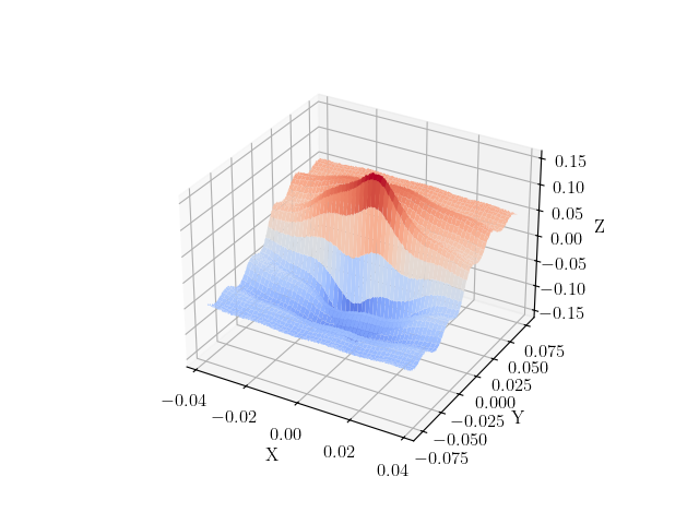
We now evaluate the function on the measured grid and add noise to it with a maximum amplitude of 2.5% of the maximum value of the function on the measured grid. We then plot the function with the added noise to verify we are producing the behavior we desire.

measured_func = analytical_function(measured_x_grid, measured_y_grid)
rng = np.random.default_rng()
noise_amp = 0.025*np.max(measured_func)
noise_multiplier = rng.random((measured_num_points, measured_num_points)) - .5
noise = noise_multiplier*noise_amp
measured_func += noise

from matplotlib import cm
fig, ax = plt.subplots(subplot_kw={"projection": "3d"})
ax.plot_surface(measured_x_grid, measured_y_grid,  measured_func,
                cmap=cm.coolwarm)
plt.xlabel("X")
plt.ylabel("Y")
ax.set_zlabel("Z")
plt.show()

With the measured data defined, we now create the simulation point cloud and the truth data for the simulation point cloud.

sim_num_points = measured_num_points
sim_xs = np.random.uniform(-W/2, W/2, sim_num_points**2)
sim_ys = np.random.uniform(-H/2, H/2, sim_num_points**2)

sim_truth_func = analytical_function(sim_xs, sim_ys)

With the measured data and truth simulation data created, we need to prepare the data to be used with the MatCal’s interface to the HWD tool. To do so, we create a FieldData object for both data sets.

measured_dict = {'x':measured_x_grid.reshape(measured_num_points**2),
                 'y':measured_y_grid.reshape(measured_num_points**2),
                 'val':measured_func.reshape(1, measured_num_points**2),
                 'time':np.array([0])}
measured_data = convert_dictionary_to_field_data(measured_dict,
                                                 coordinate_names=['x','y'])

sim_truth_dict = {'x':sim_xs,
                  'y':sim_ys,
                  'val':sim_truth_func.reshape(1, sim_num_points**2),
                  'time':np.array([0])}
sim_truth_data = convert_dictionary_to_field_data(sim_truth_dict,
                                                  coordinate_names=['x','y'])

Now we can create a set of input parameters to evaluate using our test data sets. The two input parameters to the HWD algorithm are the polynomial order of the pattern functions and the depth of subdivision tiers in the splitting tree.

To study the influence of these parameters on our mapping tool, we perform the mapping with polynomial orders of increasing polynomial orders from 1 to 8 and depths of 4 to 10.

polynomial_orders = np.array([8, 6, 4, 3, 2, 1], dtype=int) #1,2,3,4,6,8
cut_depths = np.array([10, 8, 6, 4, 2], dtype=int)#4,6,8,10
num_polys = len(polynomial_orders)
num_depths = len(cut_depths)

We then setup a function to compare the HWD weights produced from the the noisy experimental data to the HWD weights produced from the known truth data on the simulation grid. We will be using the HWDPolynomialSimulationSurfaceExtractor and HWDColocatingExperimentSurfaceExtractor classes to perform the HWD operations on our data.

Warning

The QoI extractors are not meant for direct use by users. The interfaces will likely change in future releases. Also, the names are specific for their use underneath user facing classes and may not be indicative of how they are used here.

This function requires the HWD tool input parameters of polynomial order and cut depth. It also requires that two evaluations of the function so that it can use the QoI extractors to calculate the fields and HWD weights.

from matcal.full_field.qoi_extractor import HWDColocatingExperimentSurfaceExtractor, \
     HWDPolynomialSimulationSurfaceExtractor

def get_HWD_results(poly_order, cut_depth, sim_truth_data, measured_data):
    print(f"Running Depth {cut_depth}, Order {poly_order}")
    sim_extractor = HWDPolynomialSimulationSurfaceExtractor(sim_truth_data.skeleton,
                                                            int(cut_depth), int(poly_order),
                                                            "time")
    measured_coords = measured_data.skeleton.spatial_coords[:,:2]
    sim_coords = sim_truth_data.skeleton.spatial_coords[:,:2]
    exp_extractor = HWDColocatingExperimentSurfaceExtractor(sim_extractor,
                                                            measured_coords,
                                                            sim_coords)

    measured_weights = exp_extractor.calculate(measured_data, measured_data, ['val'])
    truth_weights = sim_extractor.calculate(sim_truth_data, measured_data, ['val'], False)

    reconstructed_sim = sim_extractor._hwd._Q.dot(measured_weights['val'])
    reconstructed_error_field = (reconstructed_sim - sim_truth_data['val'])
    print(f"Depth {cut_depth}, Order {poly_order} finished.")

    return truth_weights['val'], measured_weights['val'], reconstructed_error_field

Now we can loop over the parameters, generate the HWD basis and store the values that we will be plotting next. These evaluations are computationally expensive. As a result, we use Python’s ProcessPoolExecutor to run the function in parallel for each set of HWD input parameters to speed the calculations. We also store the results in a pickle file so that they are not needlessly recalculated.

max_sim_value = np.max(np.abs(sim_truth_data['val']))
from concurrent.futures import ProcessPoolExecutor
futures = {}
with ProcessPoolExecutor(max_workers = int(num_depths*num_polys/3)) as executor:
    for p_index, poly_order in enumerate(polynomial_orders):
        futures[poly_order] = {}
        for d_index, depth in enumerate(cut_depths):
            futures[poly_order][depth] = get_HWD_results(poly_order, depth,
                                                         sim_truth_data, measured_data)
#            futures[poly_order][depth] = executor.submit(get_HWD_results,
#                                                         poly_order, depth,
#                                                         sim_truth_data, measured_data)

reconstructed_error_fields = np.zeros((num_polys, num_depths, 1,
                                       sim_truth_data.spatial_coords.shape[0]))
all_measured_weights = {}
all_truth_weights = {}
for p_index, poly_order in enumerate(polynomial_orders):
    all_measured_weights[poly_order] = {}
    all_truth_weights[poly_order] = {}
    for d_index, depth in enumerate(cut_depths):
#        results = futures[poly_order][depth].result()
        results = futures[poly_order][depth]
        all_truth_weights[poly_order][depth] = results[0]
        all_measured_weights[poly_order][depth] = results[1]
        reconstructed_error_fields[p_index,d_index]  = results[2]

Running Depth 10, Order 8

Warning: Tree depths above 8 are expensive.
Current Depth 10, which as 1024 number of subsections
Depth 10, Order 8 finished.
Running Depth 8, Order 8
Depth 8, Order 8 finished.
Running Depth 6, Order 8
Depth 6, Order 8 finished.
Running Depth 4, Order 8
Depth 4, Order 8 finished.
Running Depth 2, Order 8
Depth 2, Order 8 finished.
Running Depth 10, Order 6

Warning: Tree depths above 8 are expensive.
Current Depth 10, which as 1024 number of subsections
Depth 10, Order 6 finished.
Running Depth 8, Order 6
Depth 8, Order 6 finished.
Running Depth 6, Order 6
Depth 6, Order 6 finished.
Running Depth 4, Order 6
Depth 4, Order 6 finished.
Running Depth 2, Order 6
Depth 2, Order 6 finished.
Running Depth 10, Order 4

Warning: Tree depths above 8 are expensive.
Current Depth 10, which as 1024 number of subsections
Depth 10, Order 4 finished.
Running Depth 8, Order 4
Depth 8, Order 4 finished.
Running Depth 6, Order 4
Depth 6, Order 4 finished.
Running Depth 4, Order 4
Depth 4, Order 4 finished.
Running Depth 2, Order 4
Depth 2, Order 4 finished.
Running Depth 10, Order 3

Warning: Tree depths above 8 are expensive.
Current Depth 10, which as 1024 number of subsections
Depth 10, Order 3 finished.
Running Depth 8, Order 3
Depth 8, Order 3 finished.
Running Depth 6, Order 3
Depth 6, Order 3 finished.
Running Depth 4, Order 3
Depth 4, Order 3 finished.
Running Depth 2, Order 3
Depth 2, Order 3 finished.
Running Depth 10, Order 2

Warning: Tree depths above 8 are expensive.
Current Depth 10, which as 1024 number of subsections
Depth 10, Order 2 finished.
Running Depth 8, Order 2
Depth 8, Order 2 finished.
Running Depth 6, Order 2
Depth 6, Order 2 finished.
Running Depth 4, Order 2
Depth 4, Order 2 finished.
Running Depth 2, Order 2
Depth 2, Order 2 finished.
Running Depth 10, Order 1

Warning: Tree depths above 8 are expensive.
Current Depth 10, which as 1024 number of subsections
Depth 10, Order 1 finished.
Running Depth 8, Order 1
Depth 8, Order 1 finished.
Running Depth 6, Order 1
Depth 6, Order 1 finished.
Running Depth 4, Order 1
Depth 4, Order 1 finished.
Running Depth 2, Order 1
Depth 2, Order 1 finished.

We are interested in two error measures. The first error measure we will investigate is the L2-norm of the error field normalized by the maximum of the truth data by 100. This is a measure of the general quality of the fit for each point being evaluated and is calculated using

where are the experiment values, are the known values and is the number of values being compared. The second measure of error is the maximum error between the values from the different sources divided by the maximum of the truth data and multiplied by 100. This gives a maximum percent error for the data relative to the truth data. It is calculated using

These functions are valid for both the HWD weights and function evaluations calculated for each discretization.

The following code performs these calculations and stores the data in NumPy arrays so that they can be visualized. It also stores the data in a pickle file so that it can be read back later without recalculating since the computational cost for these calculations can be expensive.

def calculate_error_metrics(measured_fields, truth_fields=None):
    error_norms = np.zeros((num_polys, num_depths))
    error_maxes = np.zeros((num_polys, num_depths))
    for p_index, poly_order in enumerate(polynomial_orders):
        for d_index, depth in enumerate(cut_depths):
            if truth_fields:
                error_vec = (measured_fields[poly_order][depth] - truth_fields[poly_order][depth])
                val_normalization = np.max(truth_fields[poly_order][depth])
            else:
                error_vec = measured_fields[p_index,d_index].flatten()
                val_normalization = max_sim_value
            length_normalization = len(error_vec)
            error_norms[p_index, d_index] = 100 * np.linalg.norm(error_vec) / np.sqrt(length_normalization) / val_normalization
            error_maxes[p_index, d_index] = 100 * np.max(np.abs(error_vec)) / val_normalization
    return error_norms, error_maxes

weight_error_norms, weight_error_maxes = calculate_error_metrics(all_measured_weights, all_truth_weights)
field_error_norms, field_error_maxes = calculate_error_metrics(reconstructed_error_fields)

With the error fields calculated, we can now create four heat maps showing how our four error measures change as the polynomial order and cut depth are varied.

from seaborn import heatmap
import matplotlib.colors as colors

def plot_heatmap(data, title):
    heatmap(data.T,  annot=True,
            norm=colors.LogNorm(vmax=1e3),
            xticklabels=polynomial_orders,
            yticklabels=cut_depths)
    plt.title(title)
    plt.xlabel("polynomial order")
    plt.ylabel("max depth")

fig = plt.figure(figsize=(10,10), constrained_layout=True)
ax = plt.subplot(2,2,1)
plot_heatmap(weight_error_norms, "Weights $e_{{norm}}$")
ax = plt.subplot(2,2,2)
plot_heatmap(weight_error_maxes, "Weights $e_{{max}}$")
ax = plt.subplot(2,2,3)
plot_heatmap(field_error_norms, "Field $e_{{norm}}$")
ax = plt.subplot(2,2,4)
plot_heatmap(field_error_maxes, "Field $e_{{max}}$")
plt.show()

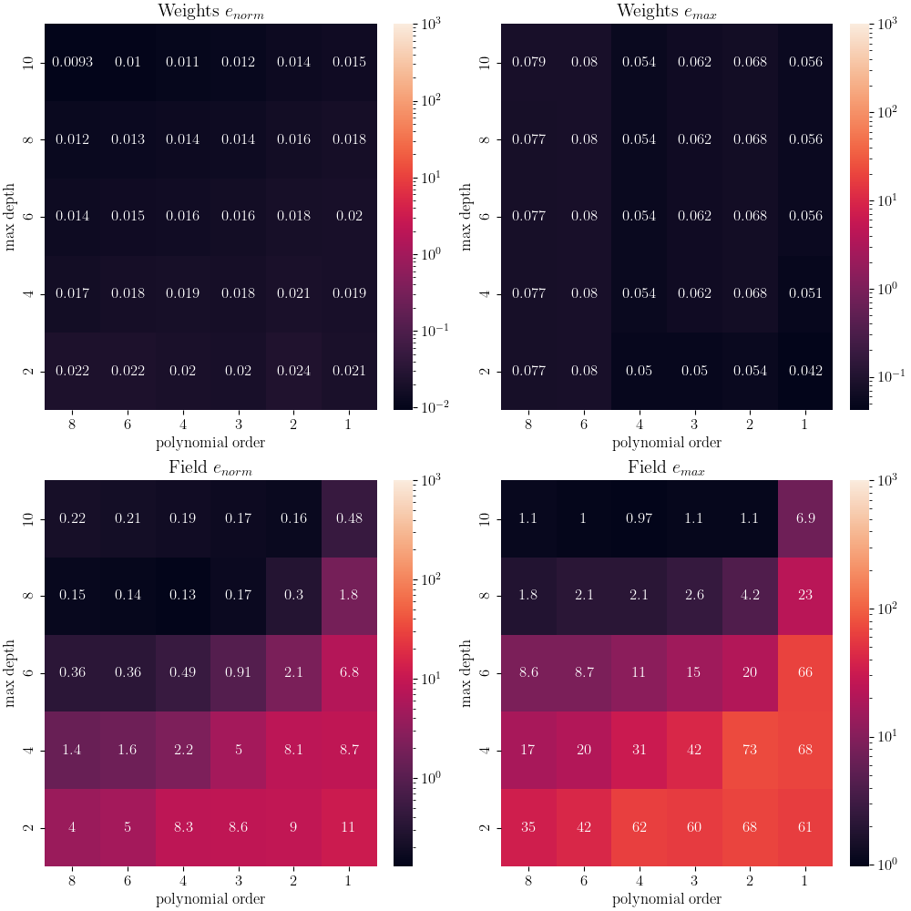
For this test, the error measures using the weights are relatively flat for all inputs. Since these fields are measured at the same points after interpolation, this is an expected result. We have shown the GMLS interpolation works well as implemented in Full-field Interpolation Verification Since the data is well interpolated, this is highlighting that we are essentially performing the same transform twice. Therefore, the error in the weights are due partially to noise and partially to interpolation error from the GMLS interpolation. It should be noted that even if the weights match for any HWD inputs, there is no guarantee that the fields will match if the HWD transform is non-unique. For low polynomial order and low cut depth HWD bases, the odds of a non-unqiue transform is higher.

As a result, we look to the error fields to determine what polynomial order and cut depth is required to adequately reconstruct the field. We visualize the produced error fields over the domain of interest for the polynomial orders of three to six and cut depths of six to ten.

poly_start_index = 1
depth_start_index = 0
viewed_polys = polynomial_orders[poly_start_index:-2]
viewed_depths =  cut_depths[depth_start_index:-2]
fig, ax_set = plt.subplots(len(viewed_polys), len(viewed_depths),
                            figsize=(5*len(viewed_depths), 5*len(viewed_polys)))
for row, po in enumerate(viewed_polys):
    ax_set[row,0].set_ylabel(f"Order: {po}")
    for col, depth in enumerate(viewed_depths):
        ax = ax_set[row, col]
        if row == 0:
            ax.set_title(f"Depth: {depth}")
        error_field = reconstructed_error_fields[row+poly_start_index,
                                                 col+depth_start_index]
        error_field = np.abs(error_field/max_sim_value*100)
        cs = ax.scatter(sim_xs, sim_ys, c=error_field.flatten(),
                        norm = colors.LogNorm(vmin=1e-2, vmax=1e1),
                        cmap='magma', marker='.', s=.9)
        ax.set_yticklabels([])
        ax.set_xticklabels([])
        ax.set_xticks([])
        ax.set_yticks([])
fig.colorbar(cs, ax=ax_set.ravel())
plt.show()

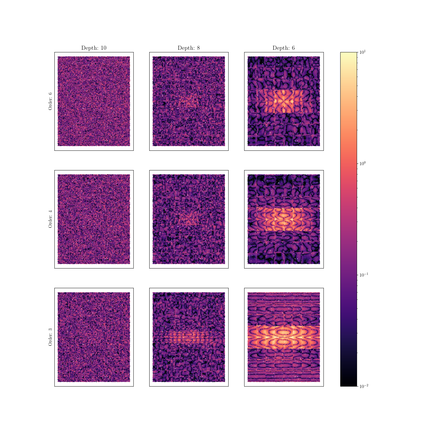
From these plots, the following conclusions can be made:

1. Recreation error is highest in the central peak region. Increasing polynomial order and depth better characterized the local behavior at this location. Increasing the depth of HWD allowed for more support of the central region. Increasing the polynomial order added additional flexibility to the wave forms allowing for a more accurate reconstruction in this area.

2. Looking at the corresponding polynomial order and depth weight errors versus the reconstruction errors, it can be seen that while it maybe possible to get good weight agreement for a wide range of polynomial-depth configurations these weights may not be capturing all of the salient features of the data. Thus configurations that have poor reconstruction error and good weight error could produce meaningful results for calibrations and VV/UQ. However, these results will only be considering what the latent space was able to capture, and thus may be missing some important parts of the data.

3. Using colocating HWD alleviates reconstruction error ‘seams’ that appear with standard HWD. This is because there is no longer any interpolation or extrapolation between point clouds. All of the data mapping is handled by the GMLS algorithm. The HWD method for this case is only providing data compression which is still useful to avoid memory issues.

Based on these findings, the recommended initial depth for an HWD calibration remains six, with a sixth order polynomial. With these settings its believed that most significant features can be captured and there will be sufficient support for the polynomial pattern functions at that level of subdivisions for most full-field data sets. If there is insufficient data for the recommended HWD configuration, then it is recommended that depth be reduced first before polynomial order.

These settings are well suited for any mapping problems that will work well for the GMLS mapping algorithm. Overall, both methods are very robust which is why colocated HWD is the default HWD method in MatCal.

Warning

Increasing either HWD parameter will increase run time and memory consumption. It may also result in regions of inadequate support which will result in a failed HWD transformation and errors in the study.

# sphinx_gallery_thumbnail_number = 2