Note
Go to the end to download the full example code.
Surrogate Generation Example
This example demonstrates how to generate a basic surrogate from a MatCal study. This example will cover:
Generating a base data set for surrogate generation
Generating a surrogate from a MatCal Study
Obtaining predictions from a surrogate
How to load a saved surrogate
How to launch an interactive window for interrogating a surrogate
The problem of interest is the uncertainty surrounding the boundary conditions for a foam and metal component in a high temperature environment. In this problem, a layer of foam separates two layers of steel. The top layer of steel is heated from a far field radiative source and convective heating from the heated gas surrounding it. We are concerned with the temperature rise immediately behind both metal layers. The temperature of the gas, the temperature of the far field source, and the speed of the ambient gas are uncertain.
This problem can be solved directly using a finite element simulation. However for large UQ analysis or complicated calibrations, the evaluation time of the finite element simulation can cause studies that require many evaluations of the model to be prohibitively long. Using surrogates as a replacement for higher-fidelity simulations offers an approach to reduce the severity of these challenges. Surrogates can enable advanced analysis techniques such as Bayesian calibration or Multi-fidelity modeling.
Surrogates in MatCal are data-based curve fits to predictions from higher fidelity simulations. As such they require an initial body (the word ‘corpus’ is often used as well) of data to be constructed, but then allow for near instant evaluation for future predictions. To generate this body of data, a large initial battery of simulations must be run. To do this in MatCal, we will run an LHS sampling study. An LHS study will allow us to efficiently sample our prediction space.
The need to run a large battery of simulations before one gets a surrogate begs the question ‘Why should I spend the time to generate a surrogate when I could just run my study with my high fidelity model?’ This is an appropriate question, for simple small analyses generating a surrogate model is not worth the upfront cost but, as the analysis gets more complicated and model evaluations more numerous, having a surrogate for relevant quantities of interest can save a lot of time. In addition, generating the body of data necessary for building a surrogate is often extremely parallelizable, thus with sufficient computing resources all of the necessary simulations can be run in a few simultaneous batches.
To generate a surrogate that predicts the heating behavior for a given set of boundary conditions, we start this example by importing MatCal and numpy.
# sphinx_gallery_thumbnail_number = 3
import matcal as mc
import numpy as np
For this example there are three parameters that define our boundary conditions. the convective heat transfer coefficient, H, relates how rapidly energy is exchanged between the ambient gas and the solid components, it is closely related to the speed of the ambient gasses. We will use it as an abstraction for how fast the gasses are moving around our component. Air values of H near 1 are characteristic of low flow environments, values near 10 are for conditions of moderate flow, and values near 100 are for conditions of strong flow. The other two parameters of interest are the temperatures of the air and a far field heat source. The ranges of these values were chosen to be on the order of temperatures seen near a fire.
conv_heat_transfer_coeff = mc.Parameter("H", 1, 100) # W / (m^2 K)
far_field_temperature = mc.Parameter("T_inf", 500, 1000) # K
air_temperature = mc.Parameter("T_air", 400, 800) # K
We then load these parameters into a Latin Hypercube Sensitivity Study. This is the
study that will be used to generate our body of training data for the surrogate.
For more details see LhsSensitivityStudy.
sampling_study = mc.LhsSensitivityStudy(conv_heat_transfer_coeff, far_field_temperature,
                                        air_temperature)
Through defining an objective for the LHS, we define what our independent and dependent fields of
interest are. In this case, we want to use ‘time’ as our independent field. Since
we do not need to compare to experimental data for this study,
we will use a SimulationResultsSynchronizer
in place of the objective. It needs the independent field,
the values of interest for the independent field and any dependent fields
of interest for the study and resulting surrogate.
When determining the independent field values of interest, it is important
to select an appropriate number of prediction points. For more complicated
physical evolutions, selecting too few points will generate poor surrogates.
n_prediction_points = 200
time_start = 0
time_end = 60 * 60 * 2
indep_field_vals = np.linspace(time_start, time_end, n_prediction_points)
my_objective = mc.SimulationResultsSynchronizer('time', indep_field_vals,
                                                 "TC_top", "TC_bottom")
Next, we need to inform MatCal about our high fidelity model. Our model is a SIERRA/aria model that we define in a local subdirectory ‘aria_model’.
my_hifi_model = mc.UserDefinedSierraModel('aria', "aria_model/metal_foam_layers.i",
                                          "aria_model/test_block.g", "aria_model/include")
my_hifi_model.set_results_filename("results/results.csv")
my_hifi_model.set_number_of_cores(2)
from site_matcal.sandia.tests.utilities import MATCAL_WCID
from site_matcal.sandia.computing_platforms import is_sandia_cluster
if is_sandia_cluster():
    my_hifi_model.run_in_queue(MATCAL_WCID, 0.25)
    my_hifi_model.continue_when_simulation_fails()
    my_hifi_model.set_number_of_cores(12)
Now we have all of our necessary components for a LHS study. We pass our model and objective into the study. We then tell our study how many cores its can use and the number of samples it needs to run. We chose 500 samples for this example because it has a decent performance floor and runs in a reasonable amount of time. Depending on the complexity of your problem, a larger sample set may be required (1000-10000).
sampling_study.add_evaluation_set(my_hifi_model, my_objective)
if is_sandia_cluster():
    sampling_study.set_core_limit(250)
else:
    sampling_study.set_core_limit(112)
sampling_study.set_number_of_samples(500)
sampling_study.set_seed(12345)
sampling_study.set_working_directory("standard_surrogate_training", remove_existing=True)
With our study defined, we run it and wait for it to complete. While it will generate information with regards to the sensitivity of the quantities of interest to the parameters, we are mostly interested in the model results the study produced.
study_results = sampling_study.launch()
Now that the study is done running, we will generate a surrogate for the model
using information stored in the study and its results.
To generate a surrogate we use MatCal’s SurrogateGenerator.
We construct a generator by passing in the study we just completed.
If we wanted to we could alter some of the surrogate generator’s settings
by evoking set_surrogate_details(),
but we pass arguments for the surrogate generator directly through its initialization.
We then generate our surrogate by
calling generate() with
a filename we would like to save our surrogate to.
The method then returns the surrogate, and saves a copy of it to
the filename we passed with a “.joblib” file extension.
surrogate_generator = mc.SurrogateGenerator(sampling_study, interpolation_field='time',
                                            regressor_type="Gaussian Process",
                                            n_restarts_optimizer=20,
                                            alpha=1e-5,
                                            normalize_y=True)
surrogate_generator.set_PCA_details(decomp_var=4)
surrogate = surrogate_generator.generate("layered_metal_bc_surrogate")
To avoid rerunning a sampling study when debugging the surrogate generator,
it is recommended that one pass a StudyResults
with the relevant information from the sampling study rather than rerun the whole
study when that is not required. This information is stored in the “final_results.joblib”
file generated by the sampling study. This information can be loaded by calling
matcal_load().
While the surrogate is being trained, the generator will report the testing and training scores for each QOI the surrogate was requested to predict. The best score for any test is 1, with poorer scores less than 1. The training score represents how well the surrogate performs on the data it was trained with, and the test score indicates how well the surrogate performs on data it was not trained on. Ideally both of these scores should be greater than .95. If either score is much below that then the surrogate will likely have poor applicability.
Warning
These scores represent how well the surrogates predict the PCA mode amplitudes not the actual curves. Therefore, adequate test scores may not be a direct indication of accuracy for predicting the response in the original space. If there are too many modes, the score may be low, but the predictions may be adequate. If there are too few modes, the score may be high, but the predictions may be poor. Always verify surrogate quality as we do below.
Even with relatively high scores, the result will likely be a decent approximation of the desired response. This can still be useful if the actual models are very expensive and you need a less expensive model to determine areas in the parameter space the produce desired results. A focused study can then be performed with the full model after using the surrogate model to identify regions of interest in the parameter space.
One important case is when the training score is much higher than the testing score. This is an indication that the surrogate is overfitting to its training data. This means that predictions outside of the training data set are likely to be very inaccurate. If this is the case there can be a couple of common causes:
The source data is poor, try increasing the number of prediction points and the number of samples run.
There is insufficient data for the underlying predictor. Increase the number of samples used during sampling and/or reduce the complexity level of the predictor.
There is a poor corelation between the QOIs and the parameters. Examine the results of the sensitivity study to gain a better understanding of how the QOIs and the parameters relate to each other and then try again.
Trying to predict QOI that change by several orders of magnitude (even going from 1 to near 0). In these cases it is better to calibrate to the natural log of these values. This can be done using the
set_fields_to_log_scale()method of the surrogate generator.
The scores are output in the log files and standard output, but can also be accessed as properties under the surrogate after it has been produced. We print the scores below for this surrogate.
print('Train scores:\n', surrogate.scores['train'])
print('Test scores:\n', surrogate.scores['test'])
Train scores:
 OrderedDict({'TC_top': 0.9999770041086106, 'TC_bottom': 0.9987124543658804})
Test scores:
 OrderedDict({'TC_top': 0.9999501576521572, 'TC_bottom': 0.9961329082917857})
Both the test scores and the training scores indicate the surrogates are well trained and can be used to predict our responses.
Now we use the surrogate to make predictions of the model
responses.
To do so, we pass in an argument list or
keyword argument list for the parameters that we want evaluated.
The surrogate will return a dictionary of predictions.
The order of the parameters is the same order that they were
passed into the the parameter collection or study, but this can be verified by
calling parameter_order().
If keyword arguments are used, the keywords must match the parameter names
assigned in the Parameter object inits.
H = 10
T_inf = 600
T_air = 400
By default, the surrogates will not allow evaluations outside of the
parameter space ranges provided in the combined test and training data sets.
Usually, the specified parameter bounds will not be included in the samples
generated from a parameter sampling study as done above. To permit evaluations at the bounds,
you can update the permissible parameter ranges using
set_parameter_ranges()
as we do below. Since we modified the surrogate, we also have to
save the surrogate so that the changes are in the stored surrogate
just in case we attempt to use it later.
surrogate.set_parameter_ranges(H=[conv_heat_transfer_coeff.get_lower_bound(),
                                  conv_heat_transfer_coeff.get_upper_bound()],
                               T_inf=[far_field_temperature.get_lower_bound(),
                                      far_field_temperature.get_upper_bound()],
                               T_air=[air_temperature.get_lower_bound(),
                                      air_temperature.get_upper_bound()])
Since we modified the surrogate, we must
save the surrogate so that the changes are in the stored surrogate
just in case we attempt to use it later.
It is saved using the matcal_save()
function.
mc.matcal_save("layered_metal_bc_surrogate.joblib", surrogate)
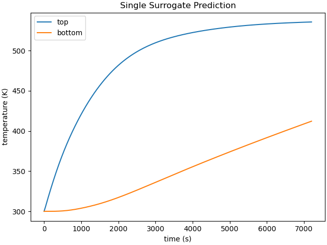
With the parameter ranges updated, we can no evaluate the surrogate with our desired parameters. This evaluation includes T_air = 400, which was the user specified bound for the training data study.
prediction = surrogate(H, T_inf, T_air)

import matplotlib.pyplot as plt
plt.close('all')
plt.figure(constrained_layout=True)
plt.plot(prediction['time'], prediction['TC_top'].flatten(), label="top")
plt.plot(prediction['time'], prediction['TC_bottom'].flatten(), label="bottom")
plt.xlabel("time (s)")
plt.ylabel("temperature (K)")
plt.legend()
plt.title("Single Surrogate Prediction")
plt.show()
Multiple sets of parameters can be evaluated simultaneously. Each field in the returned prediction will have a number of rows equal to the number of passed parameter sets. To evaluate multiple parameter sets, pass the batch_evaluate=True keyword argument
H2 = 20
T_inf2 = 815
T_air2 = 634

prediction2 = surrogate([[H, T_inf, T_air], [H2, T_inf2, T_air2]], batch_evaluate=True)
We can also run the actual model for these parameters for comparison
to the surrogate. Doing this step is recommended
when determining if a surrogate is adequate for use in calibration or
other studies. We do so using the
ParameterStudy.
param_study = mc.ParameterStudy(conv_heat_transfer_coeff, far_field_temperature,
                                 air_temperature)
param_study.add_evaluation_set(my_hifi_model, my_objective)
param_study.set_core_limit(16)
param_study.add_parameter_evaluation(H=H, T_inf=T_inf, T_air=T_air)
param_study.add_parameter_evaluation(H=H2, T_inf=T_inf2, T_air=T_air2)
results = param_study.launch()
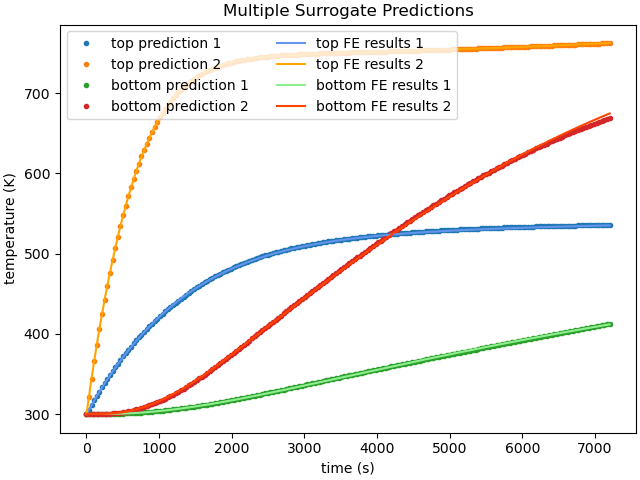
With both the finite element model results and the surrogate model results obtained, we can plot them together for comparison.
fe_data1 = results.simulation_history[my_hifi_model.name]["matcal_default_state"][0]
fe_data2 = results.simulation_history[my_hifi_model.name]["matcal_default_state"][1]


plt.figure(constrained_layout=True)
plt.plot(prediction2['time'], prediction2['TC_top'][0,:], '.', label="top prediction 1",
         color='tab:blue')
plt.plot(prediction2['time'], prediction2['TC_top'][1,:], '.', label="top prediction 2",
         color='tab:orange')
plt.plot(prediction2['time'], prediction2['TC_bottom'][0,:], '.', label="bottom prediction 1",
         color='tab:green')
plt.plot(prediction2['time'], prediction2['TC_bottom'][1,:], '.', label="bottom prediction 2",
         color='tab:red')

plt.plot(fe_data1['time'], fe_data1['TC_top'], label="top FE results 1",
         color='cornflowerblue')
plt.plot(fe_data2['time'], fe_data2['TC_top'], label="top FE results 2",
         color='orange')
plt.plot(fe_data1['time'], fe_data1['TC_bottom'], label="bottom FE results 1",
         color='lightgreen')
plt.plot(fe_data2['time'], fe_data2['TC_bottom'], label="bottom FE results 2",
         color='orangered')
plt.xlabel("time (s)")
plt.ylabel("temperature (K)")

plt.legend(ncols=2)
plt.title("Multiple Surrogate Predictions")

plt.show()
Similarly, we can plot the surrogate model error. First, we interpolate the surrogate results to the finite element model times. Next, we calculate and plot the absolute error for each prediction.
interp_prediction_top1 = np.interp(fe_data1['time'], prediction2['time'],
                                     prediction2['TC_top'][0,:])
interp_prediction_top2 = np.interp(fe_data2['time'], prediction2['time'],
                                     prediction2['TC_top'][1,:])

interp_prediction_bot1 = np.interp(fe_data1['time'], prediction2['time'],
                                     prediction2['TC_bottom'][0,:])
interp_prediction_bot2 = np.interp(fe_data2['time'], prediction2['time'],
                                     prediction2['TC_bottom'][1,:])

plt.figure(constrained_layout=True)
plt.plot(fe_data1['time'], interp_prediction_top1-fe_data1['TC_top'],
         label="top TC error 1",
         color='tab:blue')
plt.plot(fe_data2['time'], interp_prediction_top2-fe_data2['TC_top'],
         label="top TC error 2",
         color='tab:orange')
plt.plot(fe_data1['time'], interp_prediction_bot1-fe_data1['TC_bottom'],
         label="bottom TC error 1",
         color='tab:green')
plt.plot(fe_data2['time'], interp_prediction_bot2-fe_data2['TC_bottom'],
         label="bottom TC error 2",
         color='tab:red')
plt.xlabel("time (s)")
plt.ylabel("temperature error (K)")

plt.legend(ncols=2)
plt.title("Multiple Surrogate Predictions")

plt.show()
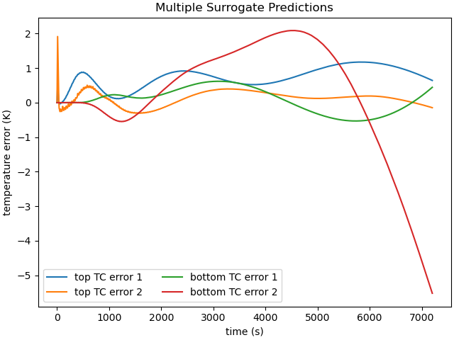
These results show that the surrogates predict the response fairly well. Most of the error is below 10 K throughout the entire history which is just a few percent for the curves. The second prediction for the bottom thermal couple has the worst surrogate prediction late in the time history. This could potentially be improved with more modes and more training samples.
If needed, we can load this surrogate again for future use by constructing a
MatCalMultiModalPCASurrogate, with the saved filename
created during the surrogate’s generation.
loaded_surrogate = mc.matcal_load("layered_metal_bc_surrogate.joblib")
loaded_prediction2 = loaded_surrogate([[H, T_inf, T_air], [H2, T_inf2, T_air2]],
                                      batch_evaluate=True)
In the follow-on examples, we compare this surrogate to adaptive surrogates. To do so, we evaluate the surrogate over a Halton sampling of the parameter space with a given seed. We then compare the maximum average error in the surrogate give 500 non-adaptive training samples to the adaptive surrogates in the other examples.
test_study = mc.HaltonStudy(conv_heat_transfer_coeff, far_field_temperature,
                                        air_temperature)
test_study.add_evaluation_set(my_hifi_model, my_objective)
test_study.set_core_limit(250)
test_study.set_number_of_samples(30)
test_study.set_seed(12345)
test_study.set_working_directory("standard_surrogate_test", remove_existing=True)
test_results = test_study.launch()
surrogate_generator.set_surrogate_details(training_fraction=1.0, test_eval_info=test_results)
surrogate = surrogate_generator.generate("layered_metal_bc_surrogate")
print(surrogate.max_errors)
OrderedDict({'train': OrderedDict({'TC_top': 5.005222870508078, 'TC_bottom': 17.061705757217737}), 'test': OrderedDict({'TC_top': 4.585223974808059, 'TC_bottom': 116.01490147862319})})
Lastly, the surrogate can be investigated in an interactive manner using MatCal’s interactive tools. To do so, use the command line call: .. code-block:: python
interactive_matcal -s <path_to_surrogate_save_file>
This command will launch a browser window in which you can investigate your surrogate.
Total running time of the script: (7 minutes 48.017 seconds)