Virtual Fields Calibration Verification

In this example, we use MatCal’s VFM tools to calibrate to the 0_degree synthetic data described in Full-field Study Verification. Due to the numerical methods used in optimization process and the errors introduced by the plane stress assumption inherent in VFM, we expect there to be some error in the parameters, An ideal result would produce calibrated parameters within a few percent of the actual values.

As we will see, this does not occur using the VFM tool with limited data.

To begin we import the MatCal tools necessary for this study and import the data that will be used for the calibration.

from matcal import *
import matplotlib.pyplot as plt

plt.rc('text', usetex=True)
plt.rc('font', family='serif')
plt.rcParams.update({'font.size': 12})

synthetic_data = FieldSeriesData("../../../docs_support_files/synthetic_surf_results_0_degree.e")

Opening exodus file: ../../../docs_support_files/synthetic_surf_results_0_degree.e
Opening exodus file: ../../../docs_support_files/synthetic_surf_results_0_degree.e
Closing exodus file: ../../../docs_support_files/synthetic_surf_results_0_degree.e
Closing exodus file: ../../../docs_support_files/synthetic_surf_results_0_degree.e

Since VFM requires a plane stress assumption, we must calibrate to portions of the data that most closely adhere to this assumption. For this problem, we must ensure that the data doesn’t include significant plastic localization. To investigate this, we plot the data load-displacement curve. If the data shows structural load loss, we know the specimen has necked.

dc = DataCollection("synthetic", synthetic_data)
dc.plot("displacement", "load")

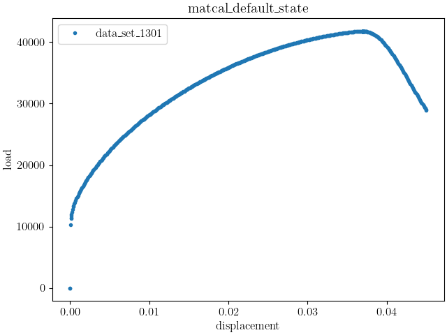
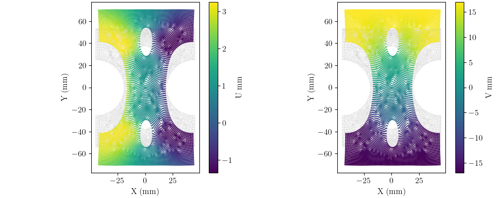
We can see peak load for this simulation occurs at a displacement of 0.036 m. Next, we remove all data past the 0.036 m displacement and then plot the X and Y displacement fields on the deformed geometry for the last time step. We plot the deformed configuration colored by the correct displacement field on top of the undeformed configuration in grey.

synthetic_data = synthetic_data[synthetic_data["displacement"] < 0.036]

import matplotlib.pyplot as plt
def plot_field(data, field, ax):
    c = ax.scatter(1e3*(data.spatial_coords[:,0]),
                   1e3*(data.spatial_coords[:,1]),
                   c="#bdbdbd", marker='.', s=1, alpha=0.5)
    c = ax.scatter(1e3*(data.spatial_coords[:,0]+data["U"][-1, :]),
                   1e3*(data.spatial_coords[:,1]+data["V"][-1, :]),
                   c=1e3*data[field][-1, :], marker='.', s=3)
    ax.set_xlabel("X (mm)")
    ax.set_ylabel("Y (mm)")
    ax.set_aspect('equal')
    fig.colorbar(c, ax=ax, label=f"{field} mm")

fig, axes = plt.subplots(1,2, figsize=(10,4), constrained_layout=True)
plot_field(synthetic_data, "U", axes[0])
plot_field(synthetic_data, "V", axes[1])
plt.show()

After importing and preparing the data, we create the VFM model that will be used to simulate the characterization test. We use a VFMUniaxialTensionHexModel for this example. This model will need a SierraSM material model input file. We create it next using python string and file tools.

mat_file_string = """begin material test_material
  density = 1
  begin parameters for model hill_plasticity
    youngs modulus  = {elastic_modulus*1e9}
    poissons ratio  = {poissons}
    yield_stress    = {yield_stress*1e6}

    hardening model = voce
    hardening modulus = {A*1e6}
    exponential coefficient = {n}

    coordinate system = rectangular_coordinate_system

    R11 = {R11}
    R22 = {R22}
    R33 = {R33}
    R12 = {R12}
    R23 = {R23}
    R31 = {R31}
  end
end
"""

with open("modular_plasticity.inc", 'w') as fn:
    fn.write(mat_file_string)

The VFM model requires a Material object. After creating the material object, we create the VFM model with the correct surface mesh that corresponds to our output surface mesh and the total specimen thickness. Next, we use the correct methods to prepare the model for the study. Most importantly we pass the correct model constants to it and pass the field data to it that includes the displacements the model will use as its boundary conditions. The model constants passed to the model are the uncalibrated parameters described in Full-field Verification Problem Material Model.

material = Material("test_material", "modular_plasticity.inc", "hill_plasticity")
vfm_model = VFMUniaxialTensionHexModel(material,
                                       "synthetic_data_files/test_mesh_surf.g",
                                       0.0625*0.0254)
vfm_model.add_boundary_condition_data(synthetic_data)
vfm_model.set_name("test_model")
vfm_model.set_number_of_cores(36)
vfm_model.set_number_of_time_steps(450)
vfm_model.set_displacement_field_names(x_displacement="U", y_displacement="V")
vfm_model.add_constants(elastic_modulus=200, poissons=0.27, R22=1.0, R33=0.9,
                        R23=1.0, R31=1.0)
from site_matcal.sandia.computing_platforms import is_sandia_cluster
from site_matcal.sandia.tests.utilities import MATCAL_WCID

if is_sandia_cluster():
    vfm_model.run_in_queue(MATCAL_WCID, 10.0/60.0)
    vfm_model.continue_when_simulation_fails()

Opening exodus file: synthetic_data_files/test_mesh_surf.g
Closing exodus file: synthetic_data_files/test_mesh_surf.g

We now create the objective that will be used for the calibration. Since our “load” and “time” fields match the default names for those fields in the MechanicalVFMObjective, no additional input is needed. We do name the objective for convenience.

vfm_objective = MechanicalVFMObjective()
vfm_objective.set_name("vfm_objective")

We then create the material model input parameters for the study. As was done in the previous examples, we provide realistic bounds that one may expect for an austenitic stainless steel based on our experience with the material. This results in an initial point far from the true values used for the synthetic data generation and is a stressing test for a local gradient based method.

Y = Parameter("yield_stress", 100, 500.0)
A = Parameter("A", 100, 4000)
n = Parameter("n", 1, 10)
R11 = Parameter("R11", 0.8, 1.1)
R12 = Parameter("R12", 0.8, 1.1)

param_collection = ParameterCollection("hill voce", Y, A, n, R11, R12)

Finally, we create the calibration study and pass the parameters relevant to the study during its initialization. We then set the total cores it can use locally and pass the data, model and objective to it as an evaluation set.

study = GradientCalibrationStudy(param_collection)
study.set_results_storage_options(results_save_frequency=len(param_collection)+1)
study.set_core_limit(48)
study.add_evaluation_set(vfm_model, vfm_objective, synthetic_data)
study.do_not_save_evaluation_cache()
study.set_working_directory("vfm_one_angle", remove_existing=True)

For this example, we limit the number of maximum evaluations. This is to save computation time. It will not converge to the correct solution with more iterations, it over fits the model to the available data and is likely traversing down a “valley” in the objective spave.

study.set_max_function_evaluations(200)
results = study.launch()

Opening exodus file: matcal_template/test_model/matcal_default_state/test_model.g
Closing exodus file: matcal_template/test_model/matcal_default_state/test_model.g
Opening exodus file: matcal_template/test_model/matcal_default_state/test_model.g
Closing exodus file: matcal_template/test_model/matcal_default_state/test_model.g
Opening exodus file: matcal_template/test_model/matcal_default_state/test_model.g
Closing exodus file: matcal_template/test_model/matcal_default_state/test_model.g
Opening exodus file: matcal_template/test_model/matcal_default_state/test_model.g
Opening exodus file: matcal_template/test_model/matcal_default_state/test_model_exploded.g
Closing exodus file: matcal_template/test_model/matcal_default_state/test_model_exploded.g
Closing exodus file: matcal_template/test_model/matcal_default_state/test_model.g

When the study completes, we extract the calibrated parameters and evaluate the error. The optimization has moved far from the initial point and provides low error for some of the parameters. It completes with RELATIVE FUNCTION CONVERGENCE indicating a quality local minima has been identified

calibrated_params = results.best.to_dict()
print(calibrated_params)

goal_results = {"yield_stress":200,
                "A":1500,
                "n":2,
                "R11":0.95,
                "R12":0.85}

def pe(result, goal):
    return (result-goal)/goal*100

for param in goal_results.keys():
    print(f"Parameter {param} error: {pe(calibrated_params[param], goal_results[param])}")

OrderedDict({'yield_stress': 193.16830661, 'A': 1526.0136645, 'n': 1.7069568852, 'R11': 0.80379719168, 'R12': 1.1})
Parameter yield_stress error: -3.4158466949999995
Parameter A error: 1.7342443000000003
Parameter n error: -14.652155739999994
Parameter R11 error: -15.389769296842104
Parameter R12 error: 29.411764705882366

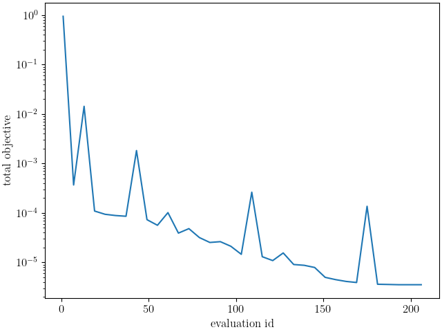
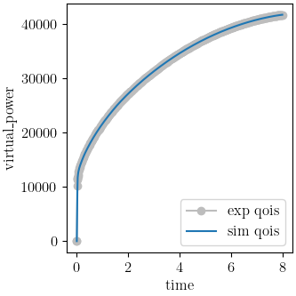
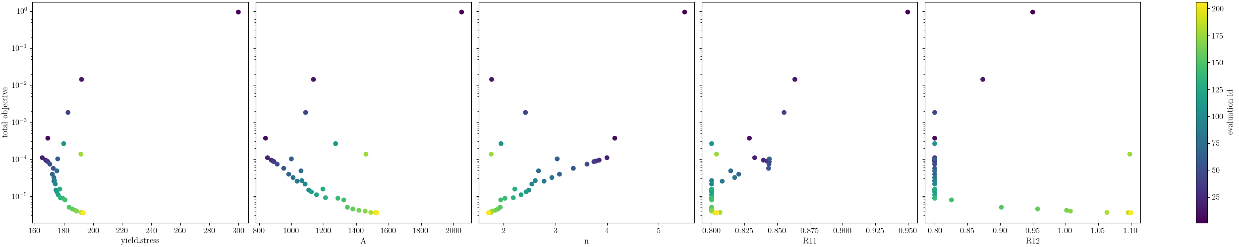
Using MatCal’s standard plot, it is clear that the gradient method quickly heads toward a minimum that is near the true values. However, once it gets to that minimum, it continues to change the parameters while the objective only decreases a small amount. This is showing that the objective has a shallow trough in this objective space. This is likely due to the model over fitting the data. The single data set is insufficient to accurately identify the parameters and the model form error allows the algorithm to continue to slowly reduce the objective by moving the parameters away from the values used to generate the synthetic data. We believe that adding data to constrain this drift will alleviate this issue. We do so in the next example Virtual Fields Calibration Verification - Three Data Sets where we see improved results.

import os
init_dir = os.getcwd()
os.chdir("vfm_one_angle")
make_standard_plots("time")
os.chdir(init_dir)

# sphinx_gallery_thumbnail_number = 5

• 
• 
•