Note
Go to the end to download the full example code.
6061T6 aluminum data analysis
In this example, we use MatCal and python tools to plot our data and verify our assumption that the material exhibits orthotropic plasticity behavior. The tests that were performed for this material that are relevant to this example include ASTME8 uniaxial tension testing in three directions relative to the material rolling direction and Sandia’s shear top hat testing [3, 4] in six orientations relative to the material rolling direction.
To use this data for calibrating the Hill48 yield surface [8], we must first define our material coordinate system. The local material directions will be denoted by numbers to adopt the convention of the Hill yield ratios in [27]. Since the material is extruded through rollers, the material coordinate system is a cartesian system aligned with the rolled plate. We decided that the material 22 direction aligns with the test rolling direction (RD), the material 11 direction will align with the long transverse direction (LT), and the material 33 direction aligns with the short transverse test direction (ST).
With the material coordinate system defined, we should determine which pairs of the six shear tests represent the same stress state for characterization of the Hill yield surface shear ratios. For each shear test, we create a free-body diagram of a material point with the test loading directions shown along with our chosen material directions. With this diagram we can see which tests are probing which shear stresses for calibrating the Hill yield shear ratios. This diagram is shown in Fig. 20.
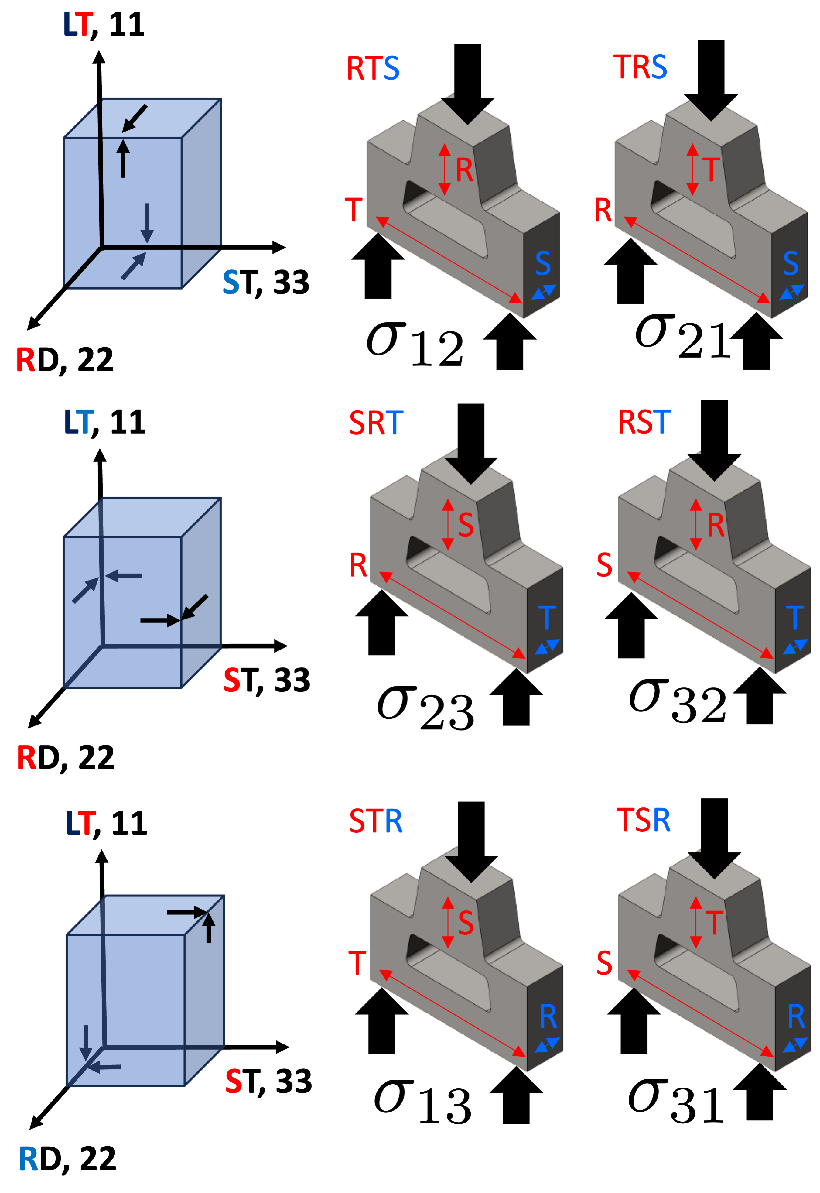
Fig. 20 The shear stress states for each test are shown here on free body diagrams of a material point on the top hat specimen where the shear bands form.
Fig. 20 shows
that the first two letters
in the test name determine the stress state
that is being probed by the test.
Since  and
and  are equal for a quasistatic material point, the stress
state is independent of the
order of the first two letters. For example, the RST and SRT
tests both impose a primarily
are equal for a quasistatic material point, the stress
state is independent of the
order of the first two letters. For example, the RST and SRT
tests both impose a primarily  /
/ stress
in the shear band and can be used to calibrate the Hill ratio
stress
in the shear band and can be used to calibrate the Hill ratio  .
As a result, we will be assigning the data one of
the three shear Hill ratios depending upon which Hill ratio they can be used to calibrate.
The RTS/TRS tests will be assigned
.
As a result, we will be assigning the data one of
the three shear Hill ratios depending upon which Hill ratio they can be used to calibrate.
The RTS/TRS tests will be assigned
R12, the SRT/RST tests will be assigned R23
and the STR/TSR tests will be assigned R31.
Similarly, the tension tests will be assigned R11, R22
and R33 for the LT, RD and ST tests, respectively.
These assignments will be done under a direction state
variable as described later in this example.
With the material directions and test names correlated to the Hill ratios, we can analyze the data and determine if we can calibrate a Hill yield surface for the material.
We begin by importing MatCal, NumPy and matplotlib, and setting global plotting options to our preferences.
import numpy as np
from matcal import *
import matplotlib.pyplot as plt
# sphinx_gallery_thumbnail_number = 3
plt.rc('text', usetex=True)
plt.rc('font', family='serif')
plt.rc('font', size=12)
figsize = (4,3)
Next, we use MatCal’s
BatchDataImporter
to import our preprocessed data files. These have been
formatted such that the importer will assign unique states to each test.
These states
are predetermined and assigned with a data preprocessing tool (not shown here).
The assignment is made by writing the state
information as the first line in each data
file according to CSV file data importing details.
This allows us to easily import the data using
the BatchDataImporter
with the correct states already assigned.
The tension data is imported first and scaled so that the units are in psi.
tension_data_collection = BatchDataImporter("aluminum_6061_data/"
                                              "uniaxial_tension/processed_data/"
                                              "cleaned_[CANM]*.csv",).batch
tension_data_collection = scale_data_collection(tension_data_collection,
                                                  "engineering_stress", 1000)
Tension testing was performed
at multiple temperatures in addition
to the multiple directions. As a result,
there are both temperature and direction state
variables for these test. To see the states
of the data sets uploaded,
print the state_names()
so that you can use these state names for manipulating the data.
print(tension_data_collection.state_names)
['temperature_5.330700e+02_direction_R11', 'temperature_5.330700e+02_direction_R22', 'temperature_5.330700e+02_direction_R33']
We then import the top hat shear data
using the BatchDataImporter.
This testing was only completed at room temperature
and only has the direction state variable.
top_hat_data_collection = BatchDataImporter("aluminum_6061_data/"
                                              "top_hat_shear/processed_data/cleaned_*.csv").batch
print(top_hat_data_collection.state_names)
['direction_R23', 'direction_R12', 'direction_R31']
Next, we use the plot()
and matplotlib tools to plot the data on two figures according to
the test geometry with their color determined by state.
tension_fig = plt.figure(figsize=figsize, constrained_layout=True)
tension_data_collection.plot("engineering_strain", "engineering_stress",
                             state="temperature_5.330700e+02_direction_R22",
                             show=False, labels="$R_{22}$", figure=tension_fig,
                             color='tab:red')
tension_data_collection.plot("engineering_strain", "engineering_stress",
                             state="temperature_5.330700e+02_direction_R11",
                             show=False, labels="$R_{11}$", figure=tension_fig,
                             color='tab:blue')
tension_data_collection.plot("engineering_strain", "engineering_stress",
                             state="temperature_5.330700e+02_direction_R33",
                             labels="$R_{33}$", figure=tension_fig,
                             color='tab:green')
tension_data_collection.remove_field("time")

top_hat_fig = plt.figure(figsize=figsize, constrained_layout=True)
top_hat_data_collection.plot("displacement", "load", show=False,
                             state="direction_R12", labels="$R_{12}$",
                             figure=top_hat_fig, color='tab:cyan')
top_hat_data_collection.plot("displacement", "load", show=False,
                             state="direction_R23", labels="$R_{23}$",
                             figure=top_hat_fig, color='tab:orange')
top_hat_data_collection.plot("displacement", "load",
                             state="direction_R31", labels="$R_{31}$",
                             figure=top_hat_fig, color='tab:purple')
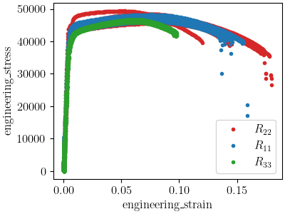
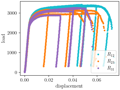
Looking at the tension stress/strain and top hat load/displacement data, it seems that the material is anisotropic. However, the material exhibits significant variability even within direction. As a result, we want a more quantitative measure from which to judge anisotropy. One way to do this is to statistically quantify differences in the stress or load at different strain or displacement values between each direction. This can be done easily using NumPy data manipulation and plotting these data with box-and-whisker plots. Since we are most interested in anisotropic yield for this material, we will look at the 0.2% offset yield stress for the tension data.
In order to look at the 0.2% offset yield values,
we need to extract those values from the data. We
do that by generating
elastic stress data with a 0.2% strain offset and determining
where these generated data
cross
the experimental data. The MatCal function
determine_pt2_offset_yield()
performs this calculation.
We can apply it to all of our data sets
and create a box-and-whisker plot comparing the yield stresses
for the different loading directions.
We do that by looping over each state in the data collection
and applying that function to each data set in each state.
We store those values in a dictionary according to state
and create the box-and-whisker plot.
yield_stresses = {"temperature_5.330700e+02_direction_R11":[],
                  "temperature_5.330700e+02_direction_R22":[],
                  "temperature_5.330700e+02_direction_R33":[]}
for state, data_sets in tension_data_collection.items():
    for data in data_sets:
        yield_pt = determine_pt2_offset_yield(data, 10e6)
        yield_stresses[state.name].append(yield_pt[1])

plt.figure(figsize=figsize, constrained_layout=True)
plt.boxplot(yield_stresses.values(), labels=["$R_{11}$", "$R_{22}$", "$R_{33}$"])
plt.xlabel("direction")
plt.ylabel("yield stress (psi)")
plt.show()
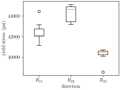
This plot shows that the median yield stress
values for the different directions are measurably
different. In fact, the medians fall outside the maximums
and minimums for the other direction data sets except for the single
outlier in the  data. Also, there
is little overlap for the different direction maximums and minimums
This plot
supports the assumption that an anisotropic
yield function should be used to model the data.
The overall
spread in the medians for the yield stress
in different directions is approximately ~10%.
data. Also, there
is little overlap for the different direction maximums and minimums
This plot
supports the assumption that an anisotropic
yield function should be used to model the data.
The overall
spread in the medians for the yield stress
in different directions is approximately ~10%.
r11_median = np.average(yield_stresses["temperature_5.330700e+02_direction_R11"])
r22_median = np.average(yield_stresses["temperature_5.330700e+02_direction_R22"])
r33_median = np.average(yield_stresses["temperature_5.330700e+02_direction_R33"])
medians = [r11_median, r22_median, r33_median]
normalized_median_range = (np.max(medians)-np.min(medians))/np.average(medians)
print(normalized_median_range)
0.09555345170158815
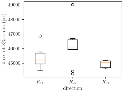
Note that there appears to be significant anisotropic hardening early in the stress strain curve. This is shown by comparing stresses at slightly higher strains. Now we create box-and-whisker plots and look at the normalized range of the medians for the engineering stress at 3% strain.
stresses = {"temperature_5.330700e+02_direction_R11":[],
                  "temperature_5.330700e+02_direction_R22":[],
                  "temperature_5.330700e+02_direction_R33":[]}
for state, data_sets in tension_data_collection.items():
    for data in data_sets:
        stress = np.interp(0.03, data["engineering_strain"], data["engineering_stress"])
        stresses[state.name].append(stress)

plt.figure(figsize=figsize, constrained_layout=True)
plt.boxplot(stresses.values(), labels=["$R_{11}$", "$R_{22}$", "$R_{33}$"])
plt.xlabel("direction")
plt.ylabel("stress at 3\% strain (psi)")
plt.show()

r11_median = np.average(stresses["temperature_5.330700e+02_direction_R11"])
r22_median = np.average(stresses["temperature_5.330700e+02_direction_R22"])
r33_median = np.average(stresses["temperature_5.330700e+02_direction_R33"])
medians = [r11_median, r22_median, r33_median]
normalized_median_range = (np.max(medians)-np.min(medians))/np.average(medians)
print(normalized_median_range)
/gpfs/knkarls/projects/matcal-stable/external_matcal/documentation/advanced_examples/6061T6_anisotropic_calibration/plot_6061T6_a_anisotropy_data_analysis.py:252: SyntaxWarning: invalid escape sequence '\%'
  plt.ylabel("stress at 3\% strain (psi)")
0.026156214170045298
We can see that the spread in the medians has reduced significantly to 2.5%. However, a measurable difference still exists. Although a more complex material model with anisotropic hardening could capture this behavior, we will continue with our chosen model form for the purpose of this example.
We now complete a similar plot for the top hat data. We will compare the load at a 0.005” displacement which is where the data appears to become nonlinear.
top_hat_yield_load = {"direction_R12":[], "direction_R23":[], "direction_R31":[]}
for state, data_sets in top_hat_data_collection.items():
    for data in data_sets:
        estimated_yield_load = np.interp(0.005, data["displacement"], data["load"])
        top_hat_yield_load[state.name].append(estimated_yield_load)

plt.figure(figsize=figsize, constrained_layout=True)
plt.boxplot(top_hat_yield_load.values(), labels=["$R_{12}$", "$R_{23}$", "$R_{31}$"])
plt.xlabel("direction")
plt.ylabel("load at 0.005\" displacement (lbs)")
plt.show()
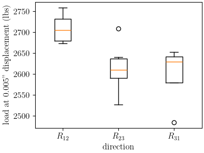
Similarly to the tension data, the top hat data also shows mild anisotropy according to this measure. With this evidence to support our material model choice, we now move on to the next example where we use this data to estimate the initial point that will be used in our full finite element calibration for the material model.
Total running time of the script: (0 minutes 4.212 seconds)