Polynomial HWD with Point Colocation Calibration Verification

This example is a repeat of the Full-field Interpolation Calibration Verification. The primary difference is that the PolynomialHWDObjective with point colocation is used instead of the InterpolatedFullFieldObjective. Since the objective function space using HWD is similar to the full-field interpolation objective as shown in Objective Sensitivity Study, we expect similar behavior but not exact replication of the results.

All other inputs and classes are the same for this calibration as they are in the full-field interpolation objective example. As a result, the commentary is mostly removed for this example except for some discussion on the results at the end.

from matcal import *
import numpy as np

synthetic_data = FieldSeriesData("../../../docs_support_files/synthetic_surf_results_0_degree.e")
synthetic_data.rename_field("U", "displacement_x")
synthetic_data.rename_field("V", "displacement_y")
synthetic_data.rename_field("W", "displacement_z")

peak_load_arg = np.argmax(synthetic_data["load"])
last_desired_arg = np.argmin(np.abs(synthetic_data["load"]\
                                    [peak_load_arg:]-np.max(synthetic_data["load"])*0.925))
synthetic_data = synthetic_data[:last_desired_arg+1+peak_load_arg]

last_disp_arg = np.argmax(synthetic_data["displacement"])
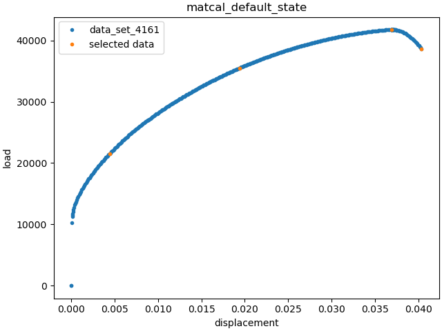
selected_data = synthetic_data[[50, 200, peak_load_arg, last_disp_arg]]
selected_data.set_name("selected data")

dc = DataCollection("synthetic", synthetic_data, selected_data)
dc.plot("displacement", "load")

import matplotlib.pyplot as plt
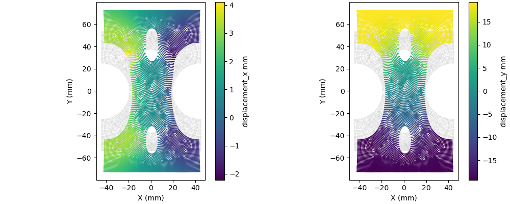
def plot_field(data, field, ax):
    c = ax.scatter(1e3*(data.spatial_coords[:,0]),
                   1e3*(data.spatial_coords[:,1]),
                   c="#bdbdbd", marker='.', s=1, alpha=0.5)
    c = ax.scatter(1e3*(data.spatial_coords[:,0]+data["displacement_x"][-1, :]),
                   1e3*(data.spatial_coords[:,1]+data["displacement_y"][-1, :]),
                   c=1e3*data[field][-1, :], marker='.', s=3)
    ax.set_xlabel("X (mm)")
    ax.set_ylabel("Y (mm)")
    ax.set_aspect('equal')
    fig.colorbar(c, ax=ax, label=f"{field} mm")

fig, axes = plt.subplots(1,2, figsize=(10,4), constrained_layout=True)
plot_field(synthetic_data, "displacement_x", axes[0])
plot_field(synthetic_data, "displacement_y", axes[1])
plt.show()

mat_file_string = """begin material test_material
  density = 1
  begin parameters for model hill_plasticity
    youngs modulus  = {elastic_modulus*1e9}
    poissons ratio  = {poissons}
    yield_stress    = {yield_stress*1e6}

    hardening model = voce
    hardening modulus = {A*1e6}
    exponential coefficient = {n}

    coordinate system = rectangular_coordinate_system

    R11 = {R11}
    R22 = {R22}
    R33 = {R33}
    R12 = {R12}
    R23 = {R23}
    R31 = {R31}
  end
end
"""

with open("modular_plasticity.inc", 'w') as fn:
    fn.write(mat_file_string)


model = UserDefinedSierraModel("adagio", "synthetic_data_files/test_model_input_reduced_output.i",
                               "synthetic_data_files/test_mesh.g", "modular_plasticity.inc")
model.set_name("test_model")
model.add_constants(elastic_modulus=200, poissons=0.27,
                    R22=1.0, R33=0.9, R23=1.0, R31=1.0)
model.read_full_field_data("surf_results.e")
from site_matcal.sandia.computing_platforms import is_sandia_cluster, get_sandia_computing_platform
from site_matcal.sandia.tests.utilities import MATCAL_WCID

num_cores=96
if is_sandia_cluster():
    model.run_in_queue(MATCAL_WCID, 0.5)
    model.continue_when_simulation_fails()
    platform = get_sandia_computing_platform()
    num_cores = platform.get_processors_per_node()
model.set_number_of_cores(num_cores)

hwd_objective = PolynomialHWDObjective("synthetic_data_files/test_mesh_surf.g", "displacement_x",
                                       "displacement_y")
hwd_objective.set_name("hwd_objective")

max_load = float(np.max(synthetic_data["load"]))
load_objective = CurveBasedInterpolatedObjective("displacement", "load", right=max_load*4)

Y = Parameter("yield_stress", 100, 500.0, 218.0)
A = Parameter("A", 100, 4000, 1863.0)
n = Parameter("n", 1, 10, 1.28)
R11 = Parameter("R11", 0.8, 1.1)
R12 = Parameter("R12", 0.8, 1.1)

param_collection = ParameterCollection("Hill48 in-plane", Y, A, n, R11, R12)

study = GradientCalibrationStudy(param_collection)
study.set_results_storage_options(results_save_frequency=len(param_collection)+1)
study.set_core_limit(100)
study.add_evaluation_set(model, load_objective, synthetic_data)
study.add_evaluation_set(model, hwd_objective, selected_data)
study.set_working_directory("hwd_cal_initial", remove_existing=True)
study.set_step_size(1e-4)
study.do_not_save_evaluation_cache()

results = study.launch()
calibrated_params = results.best.to_dict()
print(calibrated_params)

goal_results = {"yield_stress":200,
                "A":1500,
                "n":2,
                "R11":0.95,
                "R12":0.85}

def pe(result, goal):
    return (result-goal)/goal*100

for param in goal_results.keys():
    print(f"Parameter {param} error: {pe(calibrated_params[param], goal_results[param])}")

• 
• 

Opening exodus file: ../../../docs_support_files/synthetic_surf_results_0_degree.e
Opening exodus file: ../../../docs_support_files/synthetic_surf_results_0_degree.e
Closing exodus file: ../../../docs_support_files/synthetic_surf_results_0_degree.e
Closing exodus file: ../../../docs_support_files/synthetic_surf_results_0_degree.e
Opening exodus file: synthetic_data_files/test_mesh_surf.g
Closing exodus file: synthetic_data_files/test_mesh_surf.g
OrderedDict({'yield_stress': 196.17176996, 'A': 1379.0260916, 'n': 2.1086604587, 'R11': 0.97827924806, 'R12': 0.93911017046})
Parameter yield_stress error: -1.914115019999997
Parameter A error: -8.064927226666669
Parameter n error: 5.433022935000009
Parameter R11 error: 2.9767629536842146
Parameter R12 error: 10.483549465882357

The calibrated parameter percent errors are similar to those produced in the full-field interpolation objective study and the calibration completes with FALSE CONVERGENCE.

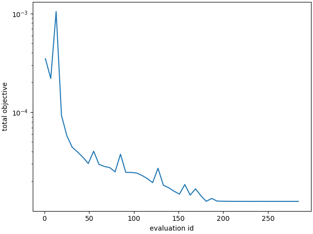
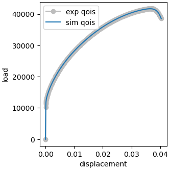
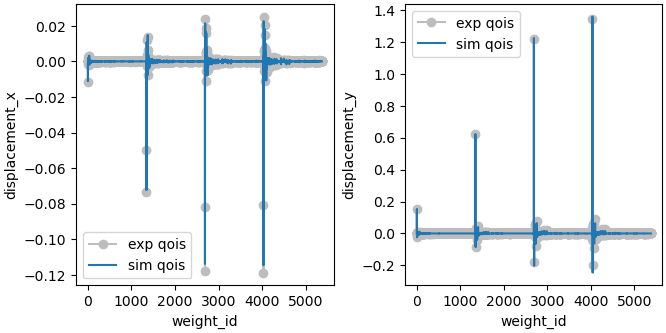
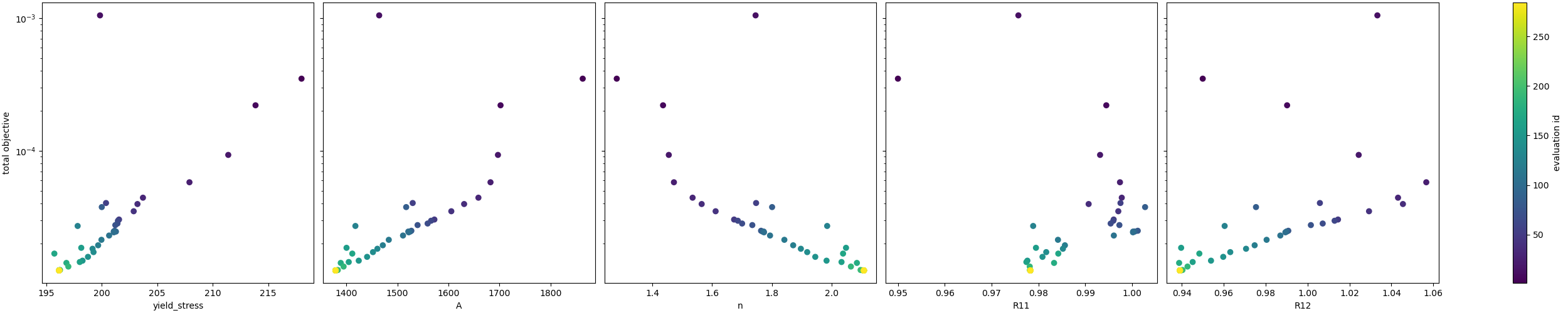
When we plot the results below, we see that the results for the load-displacement curve still agree well with the synthetic data. Also, both objectives exhibit significant reductions as the calibration progresses. As with the full-field interpolation method, the HWD objective is the cause of the improved calibration results. Also, the calibration does provide a good quality parameter set, but as with the previous example, is not accurate enough to be a verified result. In the next couple examples, we modify our objective and start with a closer initial point and see if we can obtain verification results

Note

The QoIs plotted for the HWD method re the HWD weights versus the weight_id. The weight_id is a function of time step and the mode number. The weights for all time steps are shown on a single plot.

import os
init_dir = os.getcwd()
os.chdir("hwd_cal_initial")
make_standard_plots("displacement","weight_id")
os.chdir(init_dir)


# sphinx_gallery_thumbnail_number = 5

• 
• 
• 
•