Polynomial HWD with Point Colocation Calibration Verification - 2nd Attempt

This example is a repeat of the Polynomial HWD with Point Colocation Calibration Verification with a simplification of the full-field interpolating objective.

There are two differences in this calibration that allows it to be successful where the referenced example above fails.

1. We choose to only compare data at peak load. This seems to improve the objective landscape near the true global minimum. When comparing the full-field data at multiple points in the load displacement curve, some fields may improve while others get worse. This may make the search methods unable to choose an appropriate search direction. By choosing the single step at peak load, we avoid this issue. We choose the step at peak load because it contains data where the part is highly-deformed which is relevant to the plasticity model we are calibrating

2. We choose an initial point that is only 4% away from the known solution. For this calibration we must be near the known solution for the calibration to converge using gradient methods. In real calibrations, the true solution is not known, so a non-gradient method may be needed as a first step to identify regions where the objective is lowest. Gradient calibrations can then be started from these locations to drive down to the local minima.

All other inputs remain the same. As a result, the commentary is mostly removed for this example except for some discussion on the results at the end.

from matcal import *
import numpy as np

synthetic_data = FieldSeriesData("../../../docs_support_files/synthetic_surf_results_0_degree.e")
synthetic_data.rename_field("U", "displacement_x")
synthetic_data.rename_field("V", "displacement_y")
synthetic_data.rename_field("W", "displacement_z")

peak_load_arg = np.argmax(synthetic_data["load"])
last_desired_arg = np.argmin(np.abs(synthetic_data["load"]\
                                    [peak_load_arg:]-np.max(synthetic_data["load"])*0.925))
synthetic_data = synthetic_data[:last_desired_arg+1+peak_load_arg]

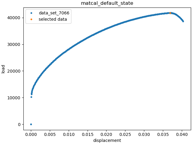
selected_data = synthetic_data[[peak_load_arg]]
selected_data.set_name("selected data")

dc = DataCollection("synthetic", synthetic_data, selected_data)
dc.plot("displacement", "load")

import matplotlib.pyplot as plt
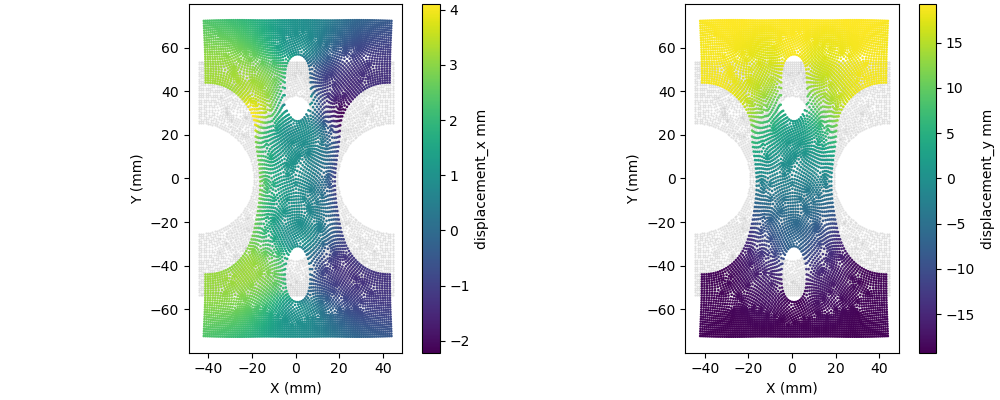
def plot_field(data, field, ax):
    c = ax.scatter(1e3*(data.spatial_coords[:,0]),
                   1e3*(data.spatial_coords[:,1]),
                   c="#bdbdbd", marker='.', s=1, alpha=0.5)
    c = ax.scatter(1e3*(data.spatial_coords[:,0]+data["displacement_x"][-1, :]),
                   1e3*(data.spatial_coords[:,1]+data["displacement_y"][-1, :]),
                   c=1e3*data[field][-1, :], marker='.', s=3)
    ax.set_xlabel("X (mm)")
    ax.set_ylabel("Y (mm)")
    ax.set_aspect('equal')
    fig.colorbar(c, ax=ax, label=f"{field} mm")

fig, axes = plt.subplots(1,2, figsize=(10,4), constrained_layout=True)
plot_field(synthetic_data, "displacement_x", axes[0])
plot_field(synthetic_data, "displacement_y", axes[1])
plt.show()

mat_file_string = """begin material test_material
  density = 1
  begin parameters for model hill_plasticity
    youngs modulus  = {elastic_modulus*1e9}
    poissons ratio  = {poissons}
    yield_stress    = {yield_stress*1e6}

    hardening model = voce
    hardening modulus = {A*1e6}
    exponential coefficient = {n}

    coordinate system = rectangular_coordinate_system

    R11 = {R11}
    R22 = {R22}
    R33 = {R33}
    R12 = {R12}
    R23 = {R23}
    R31 = {R31}
  end
end
"""

with open("modular_plasticity.inc", 'w') as fn:
    fn.write(mat_file_string)


model = UserDefinedSierraModel("adagio", "synthetic_data_files/test_model_input_reduced_output.i",
                               "synthetic_data_files/test_mesh.g", "modular_plasticity.inc")
model.set_name("test_model")
model.add_constants(elastic_modulus=200, poissons=0.27,
                    R22=1.0, R33=0.9, R23=1.0, R31=1.0)
model.read_full_field_data("surf_results.e")
from site_matcal.sandia.computing_platforms import is_sandia_cluster, get_sandia_computing_platform
from site_matcal.sandia.tests.utilities import MATCAL_WCID

num_cores=96
if is_sandia_cluster():
    model.run_in_queue(MATCAL_WCID, 0.5)
    model.continue_when_simulation_fails()
    platform = get_sandia_computing_platform()
    num_cores = platform.get_processors_per_node()
model.set_number_of_cores(num_cores)
hwd_objective = PolynomialHWDObjective("synthetic_data_files/test_mesh_surf.g", "displacement_x",
                                       "displacement_y")
hwd_objective.set_name("hwd_objective")

max_load = float(np.max(synthetic_data["load"]))
load_objective = CurveBasedInterpolatedObjective("displacement", "load", right=max_load*4)

Y = Parameter("yield_stress", 100, 500.0, 200*.96)
A = Parameter("A", 100, 4000, 1500*0.96)
n = Parameter("n", 1, 10, 2*1.04)
R11 = Parameter("R11", 0.8, 1.1, 0.95*0.96)
R12 = Parameter("R12", 0.8, 1.1, 0.85*1.04)

param_collection = ParameterCollection("Hill48 in-plane", Y, A, n, R11, R12)

study = GradientCalibrationStudy(param_collection)
study.set_results_storage_options(results_save_frequency=len(param_collection)+1)
study.set_core_limit(100)
study.add_evaluation_set(model, load_objective, synthetic_data)
study.add_evaluation_set(model, hwd_objective, selected_data)
study.set_working_directory("hwd_cal_round_2", remove_existing=True)
study.do_not_save_evaluation_cache()
study.set_step_size(1e-4)
results = study.launch()

calibrated_params = results.best.to_dict()
print(calibrated_params)

goal_results = {"yield_stress":200,
                "A":1500,
                "n":2,
                "R11":0.95,
                "R12":0.85}

def pe(result, goal):
    return (result-goal)/goal*100

for param in goal_results.keys():
    print(f"Parameter {param} error: {pe(calibrated_params[param], goal_results[param])}")

• 
• 

Opening exodus file: ../../../docs_support_files/synthetic_surf_results_0_degree.e
Opening exodus file: ../../../docs_support_files/synthetic_surf_results_0_degree.e
Closing exodus file: ../../../docs_support_files/synthetic_surf_results_0_degree.e
Closing exodus file: ../../../docs_support_files/synthetic_surf_results_0_degree.e
Opening exodus file: synthetic_data_files/test_mesh_surf.g
Closing exodus file: synthetic_data_files/test_mesh_surf.g
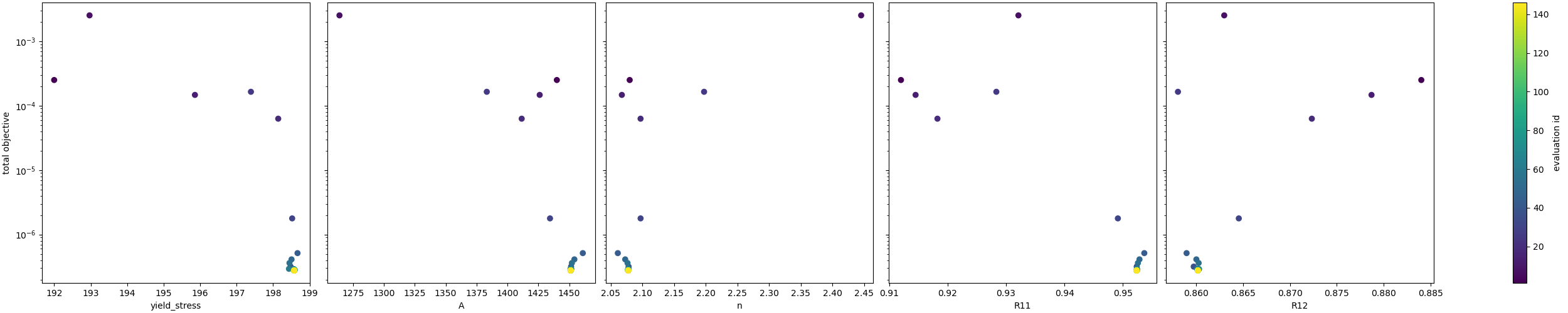
OrderedDict({'yield_stress': 198.57748613, 'A': 1451.1594729, 'n': 2.0776762488, 'R11': 0.9523697212, 'R12': 0.86019173533})
Parameter yield_stress error: -0.7112569349999944
Parameter A error: -3.2560351399999945
Parameter n error: 3.8838124400000007
Parameter R11 error: 0.2494443368421061
Parameter R12 error: 1.1990276858823603

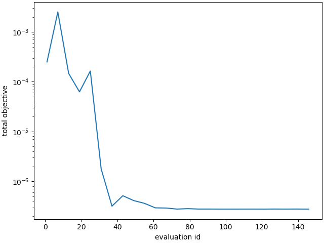
The calibration finishes with FALSE CONVERGENCE and the calibrated parameter percent errors are similar to the first attempt with HWD. This suggest improvements are needed in the objective to ensure verification quality results. However, in the presences of model form error as there is in real calibrations, the method would likely provide a calibration with satisfactory results.

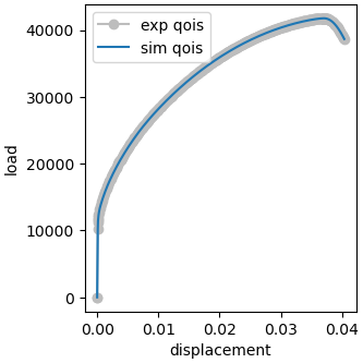
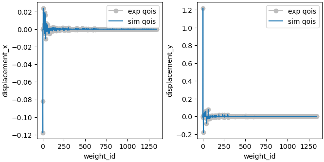
Note

The QoIs plotted for the HWD method re the HWD weights versus the weight_id. The weight_id is a function of time step and the mode number. The weights for all time steps are shown on a single plot.

import os
init_dir = os.getcwd()
os.chdir("hwd_cal_round_2")
make_standard_plots("displacement","weight_id")
os.chdir(init_dir)


# sphinx_gallery_thumbnail_number = 5

• 
• 
• 
•