Polynomial HWD Verification - X Specimen Data

In this example, we test and verify the Polynomial HWD algorithm using experimental data from [10]. We evaluate the method’s sensitivity to which point cloud is used to generate the HWD basis functions. As we will show, the choice is important and affects the validity of the HWD weights and the quality of the reconstructed fields.

This test is performed on the experimental data for one of the X specimens (XR4) and the same data that has been mapped to a simulation mesh surface using MatCal’s meshless_remapping() function.

Note

We are operating on actual data so an analytical solution is unavailable. However, our previous verification example Full-field Interpolation Verification indicated the error in mapped data should be on the order of measured noise or less. Since the noise in this data is low relative to the field of interest, most of the error that will be shown is due to the HWD field reconstruction.

We will compare these data twice, once with the experimental data as source for the basis functions and once with the mapped data as the source for these basis functions. These sets of basis functions will be referred to as the experimental basis and mapped basis, respectively. In these comparisons, we evaluate the convergence of the HWD weights for the two fields and the quality of the reconstructed fields when using the different bases.

To begin we import the libraries and tools we will be using to perform this study.

from matcal import *
import numpy as np
import matplotlib.pyplot as plt
import matplotlib.colors as colors

plt.rc('text', usetex=True)
plt.rc('font', family='serif')
plt.rcParams.update({'font.size': 12})

Next, we import the experimental data we will use for the study. We have already processed the data and extracted the field data at peak load where the displacement field is acceptably resolved with the digital image correlation (DIC) software and the geometry is highly deformed.

fields = ['V']
exp_file_data = FileData("x_specimen_XR4_peak_load_data.csv")
exp_data = convert_dictionary_to_field_data({"time":[0],
    fields[-1]:exp_file_data[fields[-1]].reshape(1, len(exp_file_data[fields[-1]]))})
spatial_coords = np.array([exp_file_data["X0"], exp_file_data["Y0"]]).T
exp_data.set_spatial_coords(spatial_coords)

Now, we import the node locations from a mesh of the geometry. The mesh has a coarser resolution of the geometry than the experimental data and covers nearly the same area.

X_sim_node_locations = FileData("sim_X_specimen_locs.csv")
X_sim_node_locations = np.array([X_sim_node_locations["X"], X_sim_node_locations["Y"]]).T

The MatCal meshless_remapping()

function is used to perform the interpolation from the experimental data points to the mesh node locations.

gmls_mapped_data = meshless_remapping(exp_data, [fields[-1]],
                                      X_sim_node_locations,
                                      polynomial_order=1,
                                      search_radius_multiplier=2.75)
gmls_mapped_data.set_spatial_coords(X_sim_node_locations)

After the interpolation, we plot the vertical displacement field V to visualize the data and the point clouds were data exists. The absolute value of the data is plotted on a log scale. This is shown to make any potential noise visible.

def plot_field(data, field, ax):
    c = ax.scatter(data.spatial_coords[:,0], data.spatial_coords[:,1],
                   c=np.abs(data[field]), marker='.', s=1,
                   norm=colors.LogNorm())
    ax.set_xlim([-0.039, 0.039])
    ax.set_ylim([-0.065, 0.065])
    ax.set_xlabel("X")
    ax.set_ylabel("Y")
    return c

fig, axes = plt.subplots(1,2, constrained_layout=True)
c =plot_field(exp_data, fields[-1], axes[0])
plot_field(gmls_mapped_data, fields[-1], axes[1])
fig.colorbar(c, ax=axes[1])
plt.show()

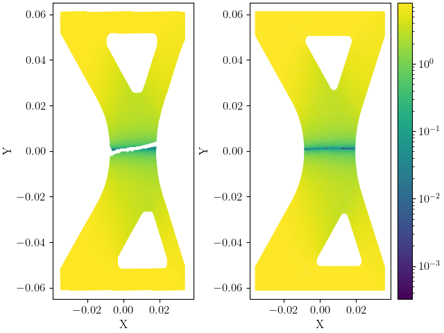
There is no clearly discernable noise in the data, but there is notable data loss near the center where the specimen has begun to plastically localize. Such data loss is inevitable and the methods should be usable even with missing points. Also, the data have been plotted in figures with the same X and Y axes limits. This was done to more clearly show that the simulation mesh covers more surface area than the data generated using the DIC software. This is an expected result due to the limitations of most common DIC software, and is not an accurate representation of the total surface geometry. The simulation mesh was built to accurately cover the total part surface assuming the part was made close to nominal dimensions and within tolerance. As we will see, the reduced area for the DIC measurement fields is the primary cause of the errors and issues that this example will highlight.

Now we create a set of input parameters to evaluate using our data sets. The two input parameters to the HWD algorithm are the polynomial order of the pattern functions and the depth of subdivision tiers in the splitting tree. To study the influence of these parameters on our mapping tool, we perform the mapping with polynomial orders 1 to 4 and depths of 4 to 8.

polynomial_orders = np.array([1, 2, 3, 4, 6, 8], dtype=int)
cut_depths = np.array( [4, 6, 8], dtype=int)
num_polys = len(polynomial_orders)
num_depths = len(cut_depths)

The MatCal tool that will be evaluated is the QoI extractor that performs the HWD operations for the PolynomialHWDObjective objective when not used with point collocation. The HWDPolynomialSimulationSurfaceExtractor is used to build the HWD basis and calculate the HWD weights for both data sets and both sets of basis functions.

Warning

The QoI extractors are not meant for direct use by users. The interfaces will likely change in future releases. Also, the names are specific for their use underneath user facing classes and may not be indicative of how they are used here.

We put the initialization of the HWD QoI extractor and calculation of our HWD weights and reconstruction into a function so that we can call it with the different HWD input parameters.

from matcal.full_field.qoi_extractor import HWDPolynomialSimulationSurfaceExtractor

def get_HWD_results(poly_order, cut_depth, basis_data, comparison_data):
    print(f"Running Depth {cut_depth}, Order {poly_order}")
    hwd_extractor = HWDPolynomialSimulationSurfaceExtractor(basis_data.skeleton,
                                                            int(cut_depth),
                                                            int(poly_order), "time")

    comparison_weights = hwd_extractor.calculate(comparison_data,
                                                 comparison_data, ['V'])
    basis_weights = hwd_extractor.calculate(basis_data, comparison_data, ['V'])

    reconstructed_field = hwd_extractor._hwd._Q.dot(comparison_weights['V'])
    reconstructed_error_field = (reconstructed_field - basis_data['V'])
    print(f"Depth {cut_depth}, Order {poly_order} finished.")
    return basis_weights['V'], comparison_weights['V'], reconstructed_error_field

We create a function that loops over the HWD method input parameters, generates the HWD basis, stores the HWD weight values and stores the reconstructed error fields for our comparison. Since we will perform these operations twice using the different basis functions sets, putting the calculations in a function simplifies the process. The following code performs these calculations and stores the data in NumPy arrays so that they can be visualized next. It also stores the data in a pickle file so that they can be loaded later without recalculating since the computational cost for these mappings can be expensive.

def evaluate_errors(basis_data, comparison_data):
    from concurrent.futures import ProcessPoolExecutor
    futures = {}
    with ProcessPoolExecutor(max_workers = num_depths*num_polys) as executor:
        for p_index,poly_order in enumerate(polynomial_orders):
            futures[poly_order] = {}
            for d_index, depth in enumerate(cut_depths):
                futures[poly_order][depth] = get_HWD_results(poly_order, depth,
                                                             basis_data,
                                                             comparison_data)

#                futures[poly_order][depth] = executor.submit(get_HWD_results,
#                                                                 poly_order, depth,
#                                                                 basis_data,
#                                                                 comparison_data)
#
    reconstructed_error_fields = np.zeros((num_polys, num_depths, 1,
                                           basis_data.spatial_coords.shape[0]))
    all_comparison_weights = []
    all_basis_weights = []
    for p_index,poly_order in enumerate(polynomial_orders):
        comparison_weights_fields_by_depth = []
        basis_weights_fields_by_depth = []
        for d_index, depth in enumerate(cut_depths):
#            results = futures[poly_order][depth].result()
            results = futures[poly_order][depth]
            basis_weights_fields_by_depth.append(results[0])
            comparison_weights_fields_by_depth.append(results[1])
            reconstructed_error_fields[p_index,d_index]  = results[2]
        all_comparison_weights.append(comparison_weights_fields_by_depth)
        all_basis_weights.append(basis_weights_fields_by_depth)

    results_dict = {"comparison weights":all_comparison_weights,
                    "basis weights":all_basis_weights,
                    "error fields":reconstructed_error_fields}
    return results_dict

exp_basis_results = evaluate_errors(exp_data, gmls_mapped_data)
mapped_basis_results = evaluate_errors(gmls_mapped_data, exp_data)

Running Depth 4, Order 1
Depth 4, Order 1 finished.
Running Depth 6, Order 1
Depth 6, Order 1 finished.
Running Depth 8, Order 1
Depth 8, Order 1 finished.
Running Depth 4, Order 2
Depth 4, Order 2 finished.
Running Depth 6, Order 2
Depth 6, Order 2 finished.
Running Depth 8, Order 2
Depth 8, Order 2 finished.
Running Depth 4, Order 3
Depth 4, Order 3 finished.
Running Depth 6, Order 3
Depth 6, Order 3 finished.
Running Depth 8, Order 3
Depth 8, Order 3 finished.
Running Depth 4, Order 4
Depth 4, Order 4 finished.
Running Depth 6, Order 4
Depth 6, Order 4 finished.
Running Depth 8, Order 4
Depth 8, Order 4 finished.
Running Depth 4, Order 6
Depth 4, Order 6 finished.
Running Depth 6, Order 6
Depth 6, Order 6 finished.
Running Depth 8, Order 6
Depth 8, Order 6 finished.
Running Depth 4, Order 8
Depth 4, Order 8 finished.
Running Depth 6, Order 8
Depth 6, Order 8 finished.
Running Depth 8, Order 8
Depth 8, Order 8 finished.
Running Depth 4, Order 1
Depth 4, Order 1 finished.
Running Depth 6, Order 1
Depth 6, Order 1 finished.
Running Depth 8, Order 1
Depth 8, Order 1 finished.
Running Depth 4, Order 2
Depth 4, Order 2 finished.
Running Depth 6, Order 2
Depth 6, Order 2 finished.
Running Depth 8, Order 2
Depth 8, Order 2 finished.
Running Depth 4, Order 3
Depth 4, Order 3 finished.
Running Depth 6, Order 3
Depth 6, Order 3 finished.
Running Depth 8, Order 3
Depth 8, Order 3 finished.
Running Depth 4, Order 4
Depth 4, Order 4 finished.
Running Depth 6, Order 4
Depth 6, Order 4 finished.
Running Depth 8, Order 4
Depth 8, Order 4 finished.
Running Depth 4, Order 6
Depth 4, Order 6 finished.
Running Depth 6, Order 6
Depth 6, Order 6 finished.
Running Depth 8, Order 6
Depth 8, Order 6 finished.
Running Depth 4, Order 8
Depth 4, Order 8 finished.
Running Depth 6, Order 8
Depth 6, Order 8 finished.
Running Depth 8, Order 8
Depth 8, Order 8 finished.

First, we will look at how the HWD weights change when using the different basis functions. We are interested in two measures for the weights. The first error measure is the L2-norm of the normalized HWD weight error field multiplied by 100. This is a general measure of how well the HWD weights are reproduced for the nearly-equivalent field when calculated from different discretizations. This error measure is calculated using

where are the weights generated from the data not used to generate the basis functions, are the weights generated from the data used to generate the basis functions and is the number of the weights generated. The second measure of error is the maximum error in the comparison field weights normalized by the maximum weight from the weights calculated for the data used to generate the basis functions. This error is also multiplied by 100 to give a maximum percent error for weights relative to the weights maximum. It is calculated using

We create a function that calculates these error metrics given the weight errors for each input parameter. We then use that function to calculate the error metrics for our two different comparisons.

def calculate_weights_error_metrics(comparison_weights, basis_weights):
    weight_error_norms = np.zeros((num_polys, num_depths))
    weight_error_maxes = np.zeros((num_polys, num_depths))
    for p_index in range(num_polys):
        for d_index in range(num_depths):
            weight_error_vec = (comparison_weights[p_index][d_index] -
                                basis_weights[p_index][d_index])
            length_normalization = len(weight_error_vec)
            val_normalization = np.max(basis_weights[p_index][d_index])
            weight_error_norms[p_index, d_index] = 100*np.linalg.norm(weight_error_vec)/ \
                np.sqrt(length_normalization)/val_normalization
            weight_error_maxes[p_index, d_index] = 100*np.max(np.abs(weight_error_vec))/ \
                val_normalization
    return weight_error_norms, weight_error_maxes

results = calculate_weights_error_metrics(exp_basis_results["comparison weights"],
                                          exp_basis_results["basis weights"])
exp_basis_weight_norms, exp_basis_weight_maxes = results
results = calculate_weights_error_metrics(mapped_basis_results["comparison weights"],
                                          mapped_basis_results["basis weights"])
sim_basis_weight_norms, sim_basis_weight_maxes = results

With the error fields calculated, we can now create two heat maps showing how our two error measures change as the polynomial order and cut depths are varied.

from seaborn import heatmap

def plot_heatmap(data, title):
    heatmap(data.T, annot=True, norm=colors.LogNorm(),
            xticklabels=polynomial_orders, yticklabels=cut_depths)
    plt.title(title)
    plt.xlabel("polynomial order")
    plt.ylabel("max depth")

fig = plt.figure(figsize=(10,10), constrained_layout=True)
ax = plt.subplot(2,2,1)
plot_heatmap(exp_basis_weight_norms, "Exp Basis $e_{{norm}}$")
ax = plt.subplot(2,2,2)
plot_heatmap(exp_basis_weight_maxes, "Exp Basis $e_{{max}}$")
ax = plt.subplot(2,2,3)
plot_heatmap(sim_basis_weight_norms, "Mapped Basis $e_{{norm}}$")
ax = plt.subplot(2,2,4)
plot_heatmap(sim_basis_weight_maxes, "Mapped Basis $e_{{max}}$")
plt.show()

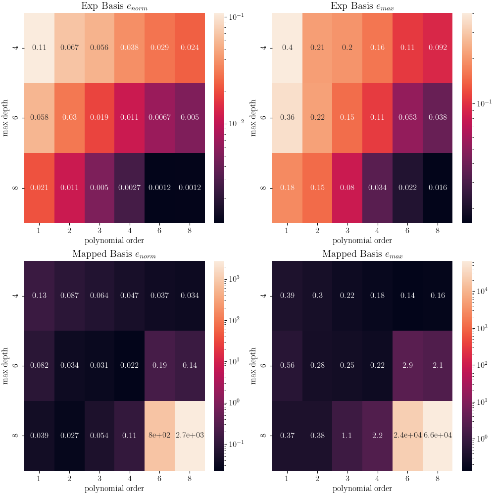
From these heat maps, it is clear that the weights match better for those generated using the experimental basis. As polynomial order and depth increases, both error metrics tend to decrease. While for the mapped basis, we see that these errors begin to get larger for higher polynomial orders and cut depths. To investigate this further, we plot the weights generated using the different basis function sets. We plot these for the combination of inputs that produced the best agreement for the weights for the experimental basis and the worst agreement for the weights the mapped basis. The inputs used to generate these weights are polynomial order six and cut depth eight for both sets of basis functions.

def setup_plot():
    plt.xlim([0,2000])
    plt.ylim([10e-6, 10e0])
    plt.ylabel("Normalized Weight")
    plt.legend()
fig = plt.figure(constrained_layout=True)
plt.subplot(2,1,1)
basis_weights = exp_basis_results["basis weights"][-1][-1]
comp_weights = exp_basis_results["comparison weights"][-1][-1]
plt.semilogy(basis_weights/np.max(basis_weights), label="exp weights")
plt.semilogy(comp_weights/np.max(basis_weights), label="mapped weights", linestyle="--")
setup_plot()
plt.title("Exp Basis")

fig = plt.figure(constrained_layout=True)
plt.subplot(2,1,2)
basis_weights = mapped_basis_results["basis weights"][-1][-1]
comp_weights = mapped_basis_results["comparison weights"][-1][-1]
plt.semilogy(comp_weights/np.max(basis_weights), label="exp weights")
plt.semilogy(basis_weights/np.max(basis_weights), label="mapped weights", linestyle="--")
setup_plot()
plt.title("Mapped Basis")
plt.show()

• 
• 

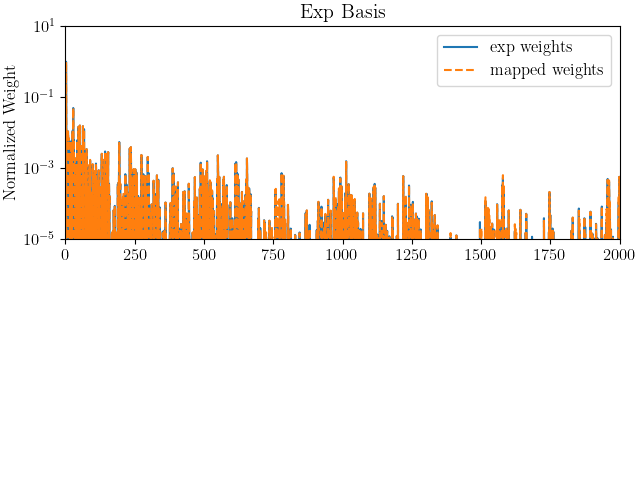
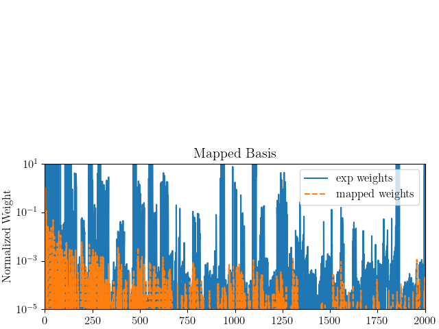
From these plots it is apparent that the experimental basis provides nearly equivalent weights for the two different discretizations and data sources. The mapped basis shows noticeable differences for most if not all modes when HWD is applied to the different data sets. To better understand why, we will plot the error fields for both the mapped and experimental bases.

These plots also indicate the level of data compression provided for the polynomial order 6 and depth cut 8 example. The full point cloud is represented by the ~2500 basis function weights and the transformation matrix which is a matrix with a size of that is governed by the number of basis functions and the number of polynomial coefficients. If the same basis functions are used for each data set, each field in the data and each time step, only the mode weights need to be stored for each time step after the initial step. This can result in significant data compression with minimal loss.

To understand the effect of the weight errors, we now visualize the error fields over the domain of interest for each set of basis functions. We do so for a reduced set of input parameters to the HWD method.

Note

The color bar scale is changing for each of these plots. When looking at the data, be cognizant of the changes to the color bar maximums and minimums.

max_value = np.max(np.abs(exp_data['V']))
def plot_error_fields(error_fields, fig_name, coords, vmax):
    poly_start_index = 2
    depth_start_index = 1
    viewed_polys = polynomial_orders[poly_start_index:]
    viewed_depths =  cut_depths[depth_start_index:]
    fig, ax_set = plt.subplots(len(viewed_polys), len(viewed_depths),
                               figsize=(5*len(viewed_depths), 5*len(viewed_polys)))
    for row, po in enumerate(viewed_polys):
        ax_set[row,0].set_ylabel(f"Order: {po}")
        for col, depth in enumerate(viewed_depths):
            ax = ax_set[row, col]
            if row == 0:
                ax.set_title(f"Depth: {depth}")
            error_field = error_fields[row+poly_start_index,
                                                    col+depth_start_index]
            error_field = np.abs(error_field/max_value*100)
            cs = ax.scatter(coords[:,0], coords[:, 1], c=error_field.flatten(),
                            norm = colors.LogNorm(vmin=1e-3, vmax=vmax),
                            cmap='magma', marker='.', s=.9)
            ax.set_yticklabels([])
            ax.set_xticklabels([])
            ax.set_xticks([])
            ax.set_yticks([])
    fig.colorbar(cs, ax=ax_set.ravel())
    plt.show()

First we observe the reconstructed field errors generated using the mapped basis and associated weights.

plot_error_fields(mapped_basis_results["error fields"], "Sim Basis Error Fields",
                  gmls_mapped_data.spatial_coords, 1e2)
plt.show()

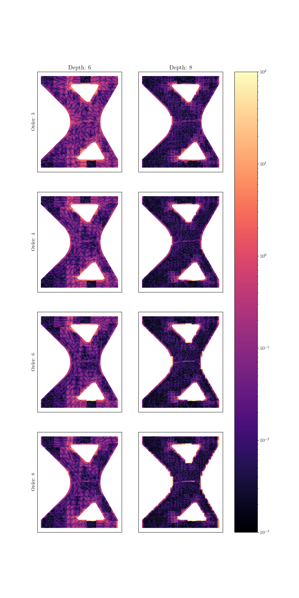
Two trends are clear.

1. As the depth increases, the largest errors isolate near edges.

2. As the polynomial order increases, this error increases significantly.

For the mapped basis, the HWD method is extrapolating near the edges where the experimental data has few points to support the polynomials. The inconsistent weight errors shown previously are, therefore, a result of extrapolation in these areas where the HWD mapped basis functions are not suitable for extrapolation given the limited points available from the experimental data. Although the linear order polynomials perform much better, they do not converge very quickly with increasing cut depth. This could be partially remedied by different domain decompositions which are an area of future research.

We now look at the same error fields for the experimental basis.

plot_error_fields(exp_basis_results["error fields"], "Exp Basis Error Fields",
                  exp_data.spatial_coords, 5)
plt.show()

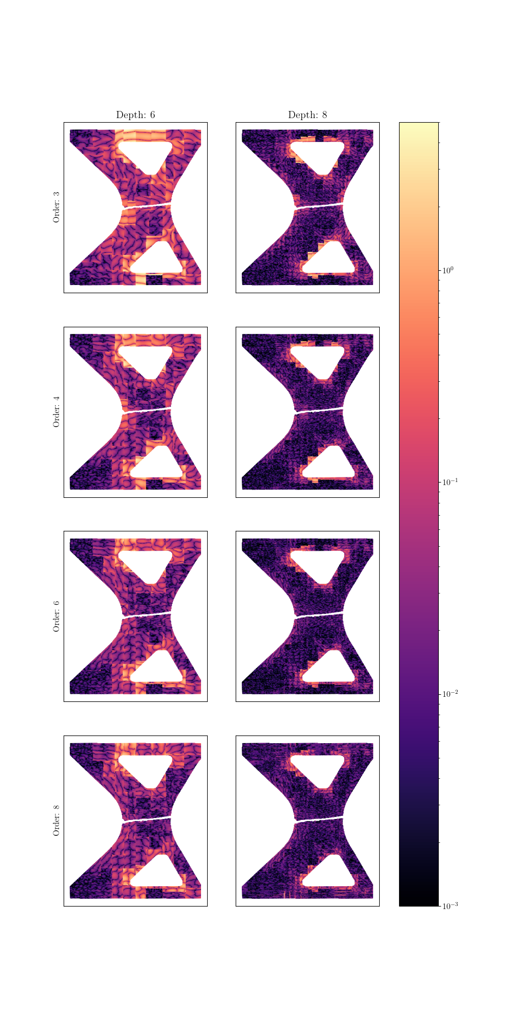
These results show that when there is enough support for the basis functions the field reconstruction performs well. However, when the smaller domain is used to generate the basis functions, extrapolation may result in large errors as the method extrapolates to points in the larger domain without sufficient support.

Since domains of different sizes are common for field data comparisons, MatCal uses our Full-field Interpolation and Extrapolation methods to move data to a common domain before using HWD methods to operate on the data. By default, we map to the simulation domain because this usually results in less memory use. With current capabilities these default settings should result in the most robust and efficient usage of the HWD tools.

Future work will involve overcoming some of these limitations to improve efficiency. Some potential solutions include:

1. Domain identification and matching. MatCal will identify the portions of the domain that do not overlap and remove them from the comparison.

2. Improved domain decomposition. MatCal will create different subsections based on the fields being analyzed, the specifics of the geometry or both.

3. Mapping the given geometry onto a simpler geometry. If geometries can be mapped to a unit square with a transformation, this would make domain decomposition trivial.

Although the potential research methods could improve efficiency to some extent, the current implementation with GMLS mapping to a common mesh is robust and provides significant memory reduction compared to comparing full-field data through interpolation alone.