Polynomial HWD Verification - Analytical Function

In this example, we use an analytical function to test and verify our use and implementation of the Polynomial HWD algorithm. We designed the verification problem to be representative of intended applications and use generate data with a function that captures much of the expected behavior seen in real data sets. We will compare the HWD weights from two point clouds populated using the function. This weights comparison is analogous to the residual calculation used in MatCal for the HWD method where we assume that a minimized difference in the HWD weights for the two discretizations of the function results in a minimized error between the two representations of the function. To show this, we will also quantify the error in an HWD reconstruction of the function against the known values of the function. For this effort, we will generate two instances of our full-field data. One will be the function sampled with added noise which is representative of experimental data. The other will be the same function evaluated at different locations without added noise. This is representative of the function being generated with a simulation with no model form error. We will complete the following steps for this example:

1. We evaluate the function on a set of points over a a predetermined domain. This will be referred to as our measurement grid and is meant to be representative of experimental data.

2. We add noise with a normal distribution to the data generated in the previous step. The noise has a maximum amplitude of 2.5% of the function maximum value to represent the noise present in measured data.

3. We create a separate domain with the same number of points from the measured grid that is unstructured and evaluate the function at these points without noise. This is to be used as the truth value of the function and this set of points will be referred to as the simulation cloud.

4. We loop over different input options to the HWD algorithm and evaluate the accuracy of the method against the truth data with five measures of error: (1) the normalized maximum percent error of the weights produced by the HWD tool, (2) the a normalized L2 norm of these weights, (3) the maximum percent error of the function reconstructed on the simulation cloud using the experimental grid HWD weights HWD, (4) the normalized L2 norm of this function and (5) plots of the reconstructed function data error for a subset of the input options studied for the HWD algorithm.

To begin we import the libraries and tools we will be using to perform this study.

from matcal import *
import numpy as np
import matplotlib.pyplot as plt

plt.rc('text', usetex=True)
plt.rc('font', family='serif')
plt.rcParams.update({'font.size': 12})

First, we defined the domain for our measured grid using NumPy tools. The domain is about 15 mm high (6 inches) and 7.6 mm wide (3 inches). The measured grid has 300 points in each dimension (x, y).

H = 6*0.0254
W = 3*0.0254

measured_num_points = 300
measured_xs = np.linspace(-W/2, W/2, measured_num_points)
measured_ys = np.linspace(-H/2, H/2, measured_num_points)

measured_x_grid, measured_y_grid = np.meshgrid(measured_xs, measured_ys)

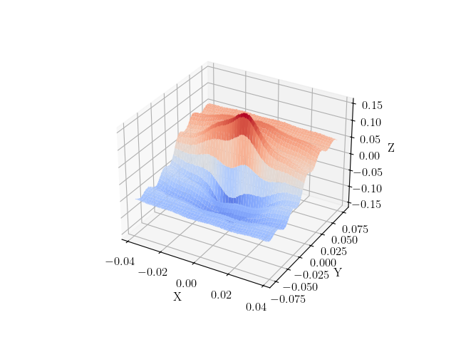
Next, we will define our test function. We are interested in generating a function that is representative of the full-field data we will use in calibrations and other MatCal studies. Generally, these data will be smooth, have some lower frequency and higher frequency behavior and may have areas of localized high gradients and values. As a result we choose, the following function which is an additive combination of three sinusoids and a linear function that is multiplied by a smooth function that approximates a dirac. This function is defined below:

def analytical_function(X,Y):
    small = H/10
    func = (H/5 * np.sin(np.pi*Y/2/(H/2)) - W/50 * X/(W/2)
           + H/40*np.sin(np.pi*Y/2/(H/20)) + W/100*np.sin(X/(W/20))) \
           * (1+small/(np.pi*(X**2+Y**2+small**2)))
    return func

We now evaluate the function on the measured grid and add noise to it with a maximum amplitude of 2.5% of the maximum value of the function on the measured grid. We then plot the function with the added noise to verify we are producing the behavior we desire.

measured_func = analytical_function(measured_x_grid, measured_y_grid)
rng = np.random.default_rng()
noise_amp = 0.025*np.max(measured_func)
noise_multiplier = rng.random((measured_num_points, measured_num_points)) - .5
noise = noise_multiplier*noise_amp
measured_func += noise

from matplotlib import cm
fig, ax = plt.subplots(subplot_kw={"projection": "3d"})
ax.plot_surface(measured_x_grid, measured_y_grid,  measured_func,
                cmap=cm.coolwarm)
plt.xlabel("X")
plt.ylabel("Y")
ax.set_zlabel("Z")
plt.show()

With the measured data defined, we now create the simulation point cloud and the truth data for the simulation point cloud.

sim_num_points = measured_num_points
sim_xs = np.random.uniform(-W/2*1.0, W/2*1.0, sim_num_points**2)
sim_ys = np.random.uniform(-H/2*1.0, H/2*1.0, sim_num_points**2)

sim_truth_func = analytical_function(sim_xs, sim_ys)

With the measured data and truth simulation data created, we need to prepare the data to be used with the MatCal’s interface to the HWD tool. To do so, we create a FieldData object for both data sets.

measured_dict = {'x':measured_x_grid.reshape(measured_num_points**2),
                 'y':measured_y_grid.reshape(measured_num_points**2),
                 'val':measured_func.reshape(1, measured_num_points**2),
                 'time':np.array([0])}
measured_data = convert_dictionary_to_field_data(measured_dict,
                                                 coordinate_names=['x','y'])

sim_truth_dict = {'x':sim_xs,
                  'y':sim_ys,
                  'val':sim_truth_func.reshape(1, sim_num_points**2),
                  'time':np.array([0])}
sim_truth_data = convert_dictionary_to_field_data(sim_truth_dict,
                                                  coordinate_names=['x','y'])

Now we can create a set of input parameters to evaluate using our test data sets. The two input parameters to the HWD algorithm are the polynomial order of the pattern functions and the depth of subdivision tiers in the splitting tree.

To study the influence of these parameters on our mapping tool, we perform the mapping with polynomial orders of increasing polynomial orders from 1 to 8 and depths of 4 to 10.

polynomial_orders = np.array([1,2,3,4,6,8], dtype=int) #1,2,3,4,6,8
cut_depths = np.array([4,6,8,10], dtype=int)#4,6,8,10
num_polys = len(polynomial_orders)
num_depths = len(cut_depths)

We then setup a function to compare the HWD weights produced from the the noisy experimental data to the HWD weights produced from the known truth data on the simulation grid. We will be using the HWDPolynomialSimulationSurfaceExtractor class to perform the HWD operations on point clouds that are not collocated.

Warning

The QoI extractors are not meant for direct use by users. The interfaces will likely change in future releases. Also, the names are specific for their use underneath user facing classes and may not be indicative of how they are used here.

This function requires the HWD tool input parameters of polynomial order and cut depth. It also requires that two evaluations of the function on the experiment grid and on the simulation cloud.

from matcal.full_field.qoi_extractor import HWDPolynomialSimulationSurfaceExtractor

def get_HWD_results(poly_order, cut_depth, sim_truth_data, measured_data):
    print(f"Running Depth {cut_depth}, Order {poly_order}")
    hwd_extractor = HWDPolynomialSimulationSurfaceExtractor(sim_truth_data.skeleton,
                                                            int(cut_depth), int(poly_order), "time")
    measured_weights = hwd_extractor.calculate(measured_data, measured_data, ['val'])
    truth_weights = hwd_extractor.calculate(sim_truth_data, measured_data, ['val'])
    reconstructed_sim = hwd_extractor._hwd._Q.dot(measured_weights['val'])
    reconstructed_error_field = (reconstructed_sim - sim_truth_data['val'])
    print(f"Depth {cut_depth}, Order {poly_order} finished.")
    return truth_weights['val'], measured_weights['val'], reconstructed_error_field

Now we can loop over the parameters, generate the HWD basis and store the values that we will be plotting next. These evaluations are computationally expensive. As a result, we use Python’s ProcessPoolExecutor to run the function in parallel for each set of HWD input parameters to speed the calculations. We also store the results in a pickle file so that they are not needlessly recalculated.

max_sim_value = np.max(np.abs(sim_truth_data['val']))
from concurrent.futures import ProcessPoolExecutor
futures = {}
with ProcessPoolExecutor(max_workers = max(num_depths*num_polys, 8)) as executor:
    for p_index,poly_order in enumerate(polynomial_orders):
        futures[poly_order] = {}
        for d_index, depth in enumerate(cut_depths):
             futures[poly_order][depth] = get_HWD_results(poly_order, depth,
                                                          sim_truth_data, measured_data)
#            futures[poly_order][depth] = executor.submit(get_HWD_results, poly_order,
#                                                         depth, sim_truth_data, measured_data)

reconstructed_error_fields = np.zeros((num_polys, num_depths, 1,
                                       sim_truth_data.spatial_coords.shape[0]))
all_measured_weights = []
all_truth_weights = []
for p_index,poly_order in enumerate(polynomial_orders):
    measured_weights_fields_by_depth = []
    truth_weights_fields_by_depth = []
    for d_index, depth in enumerate(cut_depths):
#        results = futures[poly_order][depth].result()
        results = futures[poly_order][depth]
        truth_weights_fields_by_depth.append(results[0])
        measured_weights_fields_by_depth.append(results[1])
        reconstructed_error_fields[p_index,d_index]  = results[2]
    all_measured_weights.append(measured_weights_fields_by_depth)
    all_truth_weights.append(truth_weights_fields_by_depth)

Running Depth 4, Order 1
Depth 4, Order 1 finished.
Running Depth 6, Order 1
Depth 6, Order 1 finished.
Running Depth 8, Order 1
Depth 8, Order 1 finished.
Running Depth 10, Order 1

Warning: Tree depths above 8 are expensive.
Current Depth 10, which as 1024 number of subsections
Depth 10, Order 1 finished.
Running Depth 4, Order 2
Depth 4, Order 2 finished.
Running Depth 6, Order 2
Depth 6, Order 2 finished.
Running Depth 8, Order 2
Depth 8, Order 2 finished.
Running Depth 10, Order 2

Warning: Tree depths above 8 are expensive.
Current Depth 10, which as 1024 number of subsections
Depth 10, Order 2 finished.
Running Depth 4, Order 3
Depth 4, Order 3 finished.
Running Depth 6, Order 3
Depth 6, Order 3 finished.
Running Depth 8, Order 3
Depth 8, Order 3 finished.
Running Depth 10, Order 3

Warning: Tree depths above 8 are expensive.
Current Depth 10, which as 1024 number of subsections
Depth 10, Order 3 finished.
Running Depth 4, Order 4
Depth 4, Order 4 finished.
Running Depth 6, Order 4
Depth 6, Order 4 finished.
Running Depth 8, Order 4
Depth 8, Order 4 finished.
Running Depth 10, Order 4

Warning: Tree depths above 8 are expensive.
Current Depth 10, which as 1024 number of subsections
Depth 10, Order 4 finished.
Running Depth 4, Order 6
Depth 4, Order 6 finished.
Running Depth 6, Order 6
Depth 6, Order 6 finished.
Running Depth 8, Order 6
Depth 8, Order 6 finished.
Running Depth 10, Order 6

Warning: Tree depths above 8 are expensive.
Current Depth 10, which as 1024 number of subsections
Depth 10, Order 6 finished.
Running Depth 4, Order 8
Depth 4, Order 8 finished.
Running Depth 6, Order 8
Depth 6, Order 8 finished.
Running Depth 8, Order 8
Depth 8, Order 8 finished.
Running Depth 10, Order 8

Warning: Tree depths above 8 are expensive.
Current Depth 10, which as 1024 number of subsections
Depth 10, Order 8 finished.

We are interested in two error measures. The first error measure we will investigate is the L2-norm of the error field normalized by the maximum of the truth data on the simulation cloud multiplied by 100. This is a measure of the general quality of the fit for each point being evaluated and is calculated using

where are the values being evaluated that were generated using the experimental grid points, is the known values that were generated at the simulation grid points and is the number of values generated from the simulation grid. The second measure of error is the maximum error between the values generated from the different sources divided by the maximum of the truth data and multiplied by 100. This gives a maximum percent error for the data generated from the experiment grid relative to the maximum of the data generated using the simulation cloud. It is calculated using

These functions are valid for both the HWD weights and function evaluations calculated for each discretization.

The following code performs these calculations and stores the data in NumPy arrays so that they can be visualized. It also stores the data in a pickle file so that it can be read back later without recalculating since the computational cost for these calculations can be expensive.

def calculate_error_metrics(measured_fields, truth_fields=None):
    error_norms = np.zeros((num_polys, num_depths))
    error_maxes = np.zeros((num_polys, num_depths))
    for p_index in range(num_polys):
        for d_index in range(num_depths):
            if truth_fields:
                error_vec = (measured_fields[p_index][d_index] - truth_fields[p_index][d_index])
                val_normalization = np.max(truth_fields[p_index][d_index])
            else:
                error_vec = measured_fields[p_index][d_index].flatten()
                val_normalization = max_sim_value
            length_normalization = len(error_vec)
            error_norms[p_index, d_index] = 100 * np.linalg.norm(error_vec) / np.sqrt(length_normalization) / val_normalization
            error_maxes[p_index, d_index] = 100 * np.max(np.abs(error_vec)) / val_normalization
    return error_norms, error_maxes

weight_error_norms, weight_error_maxes = calculate_error_metrics(all_measured_weights, all_truth_weights)
field_error_norms, field_error_maxes = calculate_error_metrics(reconstructed_error_fields)

With the error fields calculated, we can now create four heat maps showing how our four error measures change as the polynomial order and cut depth are varied.

from seaborn import heatmap
import matplotlib.colors as colors

def plot_heatmap(data, title):
    heatmap(data.T,  annot=True,
            norm=colors.LogNorm(vmax=1e3),
            xticklabels=polynomial_orders,
            yticklabels=cut_depths)
    plt.title(title)
    plt.xlabel("polynomial order")
    plt.ylabel("max depth")

fig = plt.figure(figsize=(10,10), constrained_layout=True)
ax = plt.subplot(2,2,1)
plot_heatmap(weight_error_norms, "Weights $e_{{norm}}$")
ax = plt.subplot(2,2,2)
plot_heatmap(weight_error_maxes, "Weights $e_{{max}}$")
ax = plt.subplot(2,2,3)
plot_heatmap(field_error_norms, "Field $e_{{norm}}$")
ax = plt.subplot(2,2,4)
plot_heatmap(field_error_maxes, "Field $e_{{max}}$")
plt.show()

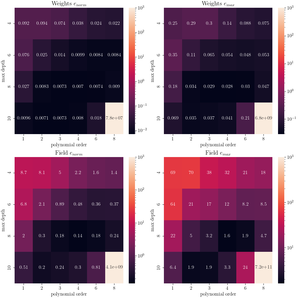
For this test, the four error measures form a minimum in a diagonal trough from the lower left near depth 10 and polynomial order 2 up to the middle right with a depth of 6 and polynomial order of 8. This is highlighting that the example function requires minimum level of flexibility in the HWD modes to fit the data. It can be achieved with either the level of cuts or the polynomial order for the HWD method. Without enough richness in the basis functions, the HWD method does a poor job representing the space and cannot uniquely identify the function on different discretizations. However, if there is too much richness as shown in the lower right corners of the heat maps, the errors show that the system is ill-conditioned. This is due to the polynomials at the lower length scales are not well supported by the number of points included in their region of support.

We now visualize the produced error fields over the domain of interest for the polynomial orders of three to six and cut depths of six to ten. We look at the error fields for these inputs to the HWD tools because most of them provide good agreement for the HWD weight error measures. The one that does not have low HWD weight error measures is the evaluation with a depth of ten and a polynomial order of six. It is shown to highlight some of the potential issues to be wary of with high depth cuts and high polynomials.

poly_start_index = 2
depth_start_index = 1
viewed_polys = polynomial_orders[poly_start_index:-1]
viewed_depths =  cut_depths[depth_start_index:]
fig, ax_set = plt.subplots(len(viewed_polys), len(viewed_depths),
                            figsize=(5*len(viewed_depths), 5*len(viewed_polys)))
for row, po in enumerate(viewed_polys):
    ax_set[row,0].set_ylabel(f"Order: {po}")
    for col, depth in enumerate(viewed_depths):
        ax = ax_set[row, col]
        if row == 0:
            ax.set_title(f"Depth: {depth}")
        error_field = reconstructed_error_fields[row+poly_start_index,
                                                 col+depth_start_index]
        error_field = np.abs(error_field/max_sim_value*100)
        cs = ax.scatter(sim_xs, sim_ys, c=error_field.flatten(),
                        norm = colors.LogNorm(vmin=1e-2, vmax=1e1),
                        cmap='magma', marker='.', s=.9)
        ax.set_yticklabels([])
        ax.set_xticklabels([])
        ax.set_xticks([])
        ax.set_yticks([])
fig.colorbar(cs, ax=ax_set.ravel())
plt.show()

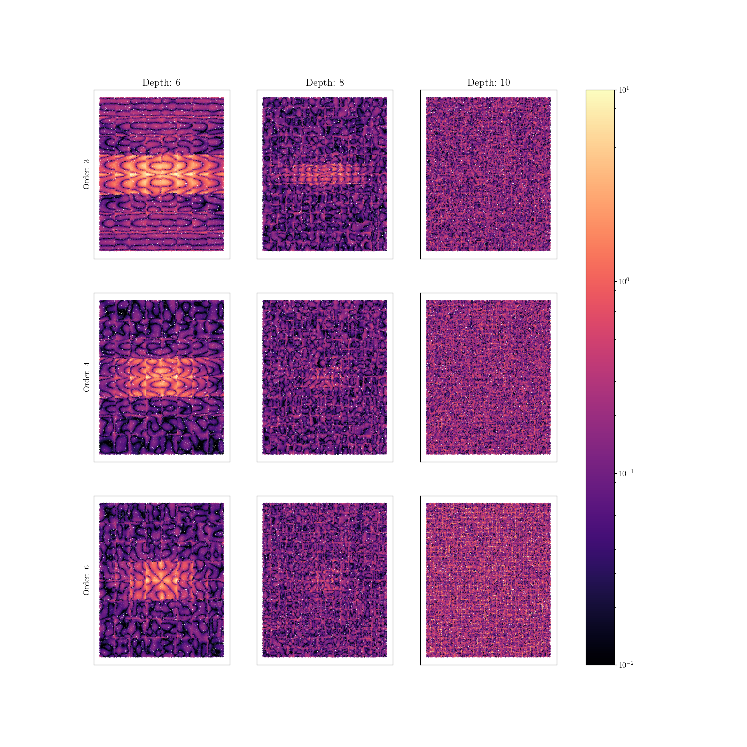
From these plots, the following conclusions can be made:

1. Recreation error is highest in the central peak region. Increasing polynomial order and depth better characterized the local behavior at this location. Increasing the depth of HWD allowed for more support of the central region. Increasing the polynomial order added additional flexibility to the wave forms allowing for a more accurate reconstruction in this area.

2. Looking at the corresponding polynomial order and depth weight errors versus the reconstruction errors, it can be seen that while it maybe possible to get good weight agreement for a wide range of polynomial-depth configurations these weights may not be capturing all of the salient features of the data. Thus configurations that have poor reconstruction error and good weight error could produce meaningful results for calibrations and VV/UQ. However, these results will only be considering what the latent space was able to capture, and thus may be missing some important parts of the data.

3. The subdivision selection used in HWD misses important aspects of the data. In the reconstruction error ‘seams’ can be seen that indicate the different subdivisions created by HWD. These do not seem to be arranged in a fashion that would allow the pattern functions to create the best basis possible. This is to be expected because of the purely geometry based decomposition method existing within the HWD library.

Based on these findings, the recommended initial depth for an HWD calibration is six, with a sixth order polynomial. With these settings its believed that most significant features can be captured and there will be sufficient support for the polynomial pattern functions at that level of subdivisions for most full-field data sets. If there is insufficient data for the recommended HWD configuration, then it is recommended that depth be reduced first before polynomial order.

These settings are best suited for mapping problems with the following characteristics:

1. The underlying function being studied is relatively smooth when compared to the discretization point cloud spacing. In other words, the point cloud spacing should be significantly smaller than the size of the features of interest for the function that they hold data for.

2. The data being compared is not extrapolated. The higher order polynomials and small areas of support will lead to large extrapolation errors.

If the data set is not smooth, then higher order polynomials may create a worse representation of the data. In these cases it is better to reduce the polynomial orders used and increase the depth of the HWD tree. This will allow the representation to better align with rough or discontinuous data. In addition, while HWD has great potential to capture discontinuous data patterns, it does this best when subdivision lines coexist with regions of discontinuous behavior. Improving the geometric decomposition of the domain is planned planned for future releases.

Warning

Increasing either HWD parameter will increase run time and memory consumption. It may also result in regions of inadequate support which will result in a failed HWD transformation and errors in the study.

# sphinx_gallery_thumbnail_number = 2