Successful Calibration

As stated previously, we present the calibration of our UniaxialLoadingMaterialPointModel to uniaxial compression data for a 6061-T6 aluminum from the Ductile Failure Project at Sandia [13]. This example and calibration will consist of three steps:

1. Data overview, analysis and preprocessing.

2. Model selection and preparation.

3. Calibration execution and results review.

To begin, import all of MatCal’s calibration tools:

# sphinx_gallery_thumbnail_number = 5

from matcal import *
import matplotlib.pyplot as plt
plt.rc('text', usetex=True)
plt.rc('font', family='serif')
plt.rc('font', size=12)
figsize = (4,3)

Next we will review the data for model calibration. For the UniaxialLoadingMaterialPointModel, we support only specific data fields for calibration. These are ‘time’, ‘engineering_strain’, ‘engineering_stress’, ‘true_strain’, ‘true_stress’ and ‘contraction’. To learn more see Uniaxial Loading Material Point Model. For this calibration, we will be using true stress and strain data for the calibration. This data is used for both the objective calculation and boundary condition generation. To load the data, we can use the BatchDataImporter tool that imports data from multiple files. It puts the data into a DataCollection which has a basic plotting method plot() for simple visualization and debugging.

data_collection = BatchDataImporter("uniaxial_material_point_data/*.csv").batch
data_collection.plot("true_strain", "true_stress")
data_collection.plot("time", "true_strain")

• 
• 

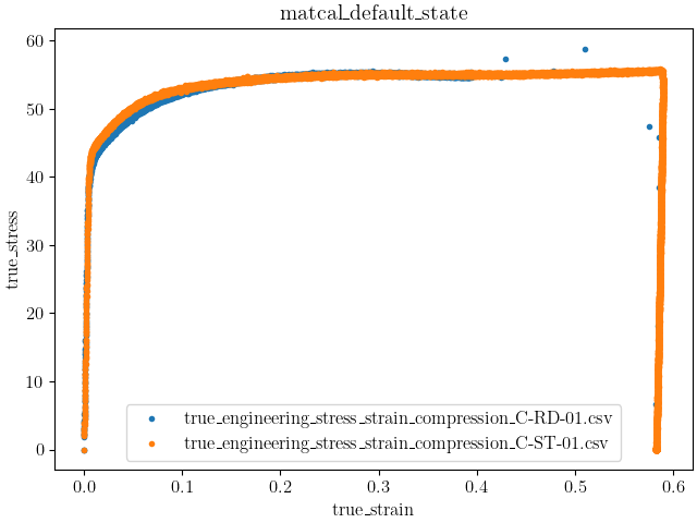
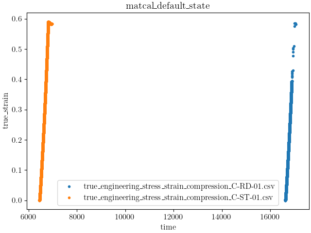
It is clear from the data that the test specimens’ ‘time’ data fields do not have a common start time. Although this is not necessarily an issue for MatCal’s UniaxialLoadingMaterialPointModel, it does makes visualizing the data inconvenient. Since the Data class is derived from NumPy arrays [7], it is easy to modify the data for convenient viewing.

for state_data_list in data_collection.values():
  for data in state_data_list:
    data['time'] = data['time'] - data['time'][0]
data_collection.plot("time", "true_strain")

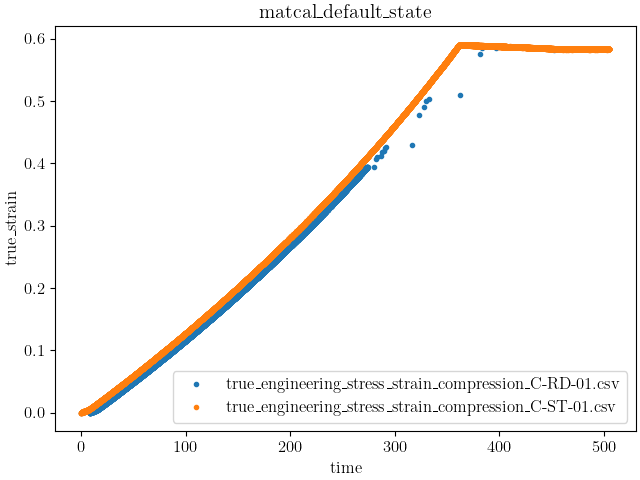
With the updated plots, two features are evident:

1. Dataset C-RD-01 appears to have gone unstable in some fashion and

2. Dataset C-ST-01 has a period of unloading.

These features are important to take note of due to how MatCal will produce boundary conditions for its UniaxialLoadingMaterialPointModel. The UniaxialLoadingMaterialPointModel has a method add_boundary_condition_data() that is used to provide data for boundary condition determination for the model. This boundary condition determination is done by state since maximum deformation, material behavior and experiment setup can vary significantly over different states. These boundary conditions are determined from the data according to the following:

1. Find the data in each state with the largest strain. This dataset will be used to produce the boundary condition function.

2. If ‘time’ and ‘engineering_strain’ or ‘true_strain’ data exists for the chosen dataset, use this as the direct input strain function for the model. The model currently only uses engineering strain input, so true strain data is converted to engineering strain which is then applied to the model as an appropriately scaled displacement function.

3. If ‘engineering_strain’ and ‘true_strain’ are fields for the data set, use the ‘engineering_strain’ field for the boundary condition. Otherwise, if only ‘true_strain’ is available, convert it to engineering strain and use it for the boundary condition.

4. If ‘time’ is not in the data, but the state has a state variable named ‘engineering_strain_rate’. Apply engineering strain linearly at the given state engineering strain rate until the model has reached the maximum strain measured for that state.

5. If ‘time’ is not in the data and no ‘engineering_strain_rate’ state variable is present, deform the model from no strain to the maximum strain over 1 second.

Warning

If both true strain and engineering strain exist in the data, it will default to using the engineering strain data to create the boundary condition. As a result, any changes applied to the true strain data in an effort to modify the model boundary conditions should also be done to the engineering strain data. In most cases, if modifying the true strain data for boundary condition purposes, it is best to remove the engineering strain from the data if both are present in the data to begin with. MatCal will automatically generate an engineering strain data field from the true strain data field.

Note

The Data or DataCollection used for boundary condition generation does not need to be the same as that use for calibration. As a result, custom boundary condition data can be generated by the user for more complex load cases. See convert_dictionary_to_data().

Note

Compression boundary conditions are supported and must be passed as negative strain values to the model. If compression is used, the model will output negative stresses. If compression data is provided from the source with positive stress/strain values use scale_data_collection() to convert the data to negative stress/strain.

Based on this information, we will choose to force the dataset C-ST-01 to be used as the data for boundary condition generation. To do so, we will create a new data class that consists of a NumPy view into a subset of the dataset. We do this by first selecting the dataset from our DataCollection which is indexed first by State or name(). and the order in which the data was added to the data collection. In this case no state is defined, so the default state name “matcal_default_state” is used. The data are then added to the DataCollection by sorting based on the filename, so we will select the data at index location 1. Next, we use NumPy array slicing to manipulate the data and feed only the data that are required to the model for boundary condition generation. In this case the model only needs the engineering strain field from the data of choice since we do not need to simulate the loading history with this model form. When only the engineering strain data is provided for boundary condition generation, the model will be deformed from no deformation to the maximum strain in the data for the state of interest in 1 second. Finally, since this data was taken in compression, we need to convert the data to negative strains so that it is interpreted correctly during boundary condition generation.

boundary_data = data_collection["matcal_default_state"][1]
boundary_data = boundary_data[["engineering_strain"]]
boundary_data.set_name("dataset 1 derived BC data")
boundary_data_collection = DataCollection('boundary_data', boundary_data)
boundary_data_collection = scale_data_collection(boundary_data_collection, "engineering_strain", -1)

Note

With the current model form, the model will produce the same result whether in compression or tension as long as the proper boundary condition is produced. The data is converted to compression here to demonstrate that compression data can be used to create compressive models and, since we a working with engineering strains, compression is required. Correctly modeling compressive or tensile stress states is required for models with tension/compression asymmetry, and is considered good practice for all cases.

data_collection = scale_data_collection(data_collection, "true_strain", -1)
data_collection = scale_data_collection(data_collection, "true_stress", -1000)

With the boundary condition data chosen, we can now analyze the data to choose a model form for calibration. The data show that after yield the material hardens before the hardening rate reduces and eventually a saturation stress is reached. As a result, we choose to calibrate a J2 plasticity model with Voce hardening to the material model which should match the data well. The flow rule is defined by:

where is the material yield, is the Voce hardening modulus, is the Voce exponent, and is the material plastic strain. As with any plasticity model, when the flow stress is greater than the equivalent stress, which is the von Mises stress for this material, plastic flow occurs. We will need to calibrate the , , and parameters.

Y = Parameter('Y', 30, 60, 50)
A = Parameter('A', 1, 500, 100)
b = Parameter('b', 5, 30, 20)

Now we can create a Material class and corresponding material file for the calibration. The input deck for this material model in SIERRA/SM is shown below:

begin material j2_voce
  density = 0.000254
  begin parameters for model j2_plasticity
    youngs modulus                = 9.9e6
    poissons ratio                =   0.33
    yield stress                  = {Y*1e3}

    hardening model = voce
    hardening modulus = {A*1e3}
    exponential coefficient = {b}
   end
end

The material that we are calibrating is a 6061-T6 aluminum. The elastic properties and density can be pulled from the literature. In this case we use values provided by MMPDS10 [1]. With this SIERRA/SM input saved in the current directory as “sierra_sm_voce_hardening.inc”, we can create the Material and the UniaxialLoadingMaterialPointModel.

j2_voce = Material("j2_voce", "sierra_sm_voce_hardening.inc", "j2_plasticity")

mat_point_model = UniaxialLoadingMaterialPointModel(j2_voce)
mat_point_model.add_boundary_condition_data(boundary_data_collection)
mat_point_model.set_name("compression_mat_point")

Next the parameters are passed to a study. In this case, we will use a GradientCalibrationStudy to perform the calibration. For this simple set of data and simple model, this type of study will work well.

calibration = GradientCalibrationStudy(Y, A, b)
calibration.set_results_storage_options(results_save_frequency=4)

The last component needed for the calibration is an objective to minimize. For this calibration, we will use a CurveBasedInterpolatedObjective that matches the true stress/strain curve generated using the model to the experimental data collected.

objective = CurveBasedInterpolatedObjective('true_strain','true_stress')

Warning

The CurveBasedInterpolatedObjective expects the independent data field to be monotonically increasing since it is uses the NumPy interp method to interpolate the simulation data to the experiment data independent field locations. To support negative data, MatCal sorts the data so that the independent variable is monotonically increasing to meet this requirement. Be sure your data will behave as intended when passed to this objective.

One more step remains before this objective is ready for use in the calibration. Since the material data being used for the calibration has unloading data and our model does not, we must modify the objective or the data to remove this data from the calibration. With the objective we are using, we do not want to modify the QoI Extractor since this objective has a predefined extractor for interpolation. We also want to keep the entire original dataset. This leaves us with the option to use a weighting function that modifies the residuals such that the unloading points do not affect the objective. We also should remove the elastic loading portion of the curve. Since we are not calibrating the elastic parameters, it should not contribute to the residual. Furthermore, since this portion of the curve is steep, even small errors in the slope could lead to large contribution to the objectives. Therefore, to ensure the objective provides the calibration we want, we use a UserFunctionWeighting to ensure only the data we want to use for calibration affects the objective. To do so, we define a function that performs the residual weighting. Once again, we can leverage NumPy array slicing to select the data we wish to exclude and set their weights to zero, effectively removing their influence on the objective.

def remove_high_and_low_strain_from_residual(true_strains, true_stresses, residuals):
    import numpy as np
    weights = np.ones(len(residuals))
    weights[(-true_strains > 0.5) | (-true_strains < 0.0035)] = 0
    return weights*residuals

residual_weights = UserFunctionWeighting("true_strain", "true_stress",
                                         remove_high_and_low_strain_from_residual)

objective.set_field_weights(residual_weights)

To learn more about matcal.core.residuals.UserFunctionWeighting please view its documentation. With the model, objective and data defined, we can now give the study an evaluation set. These evaluation sets give the study all pieces needed to evaluate an objective essentially tying a dataset, model and objective together for evaluation. Although multiple evaluation sets can be added to a study, only one is needed for this basic calibration.

calibration.add_evaluation_set(mat_point_model, objective, data_collection)

The last step is to launch the calibration study and review the results.

calibration.set_core_limit(4)
results = calibration.launch()
print(results.best.to_dict())
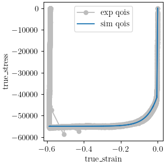
make_standard_plots("true_strain")

• 
• 
• 

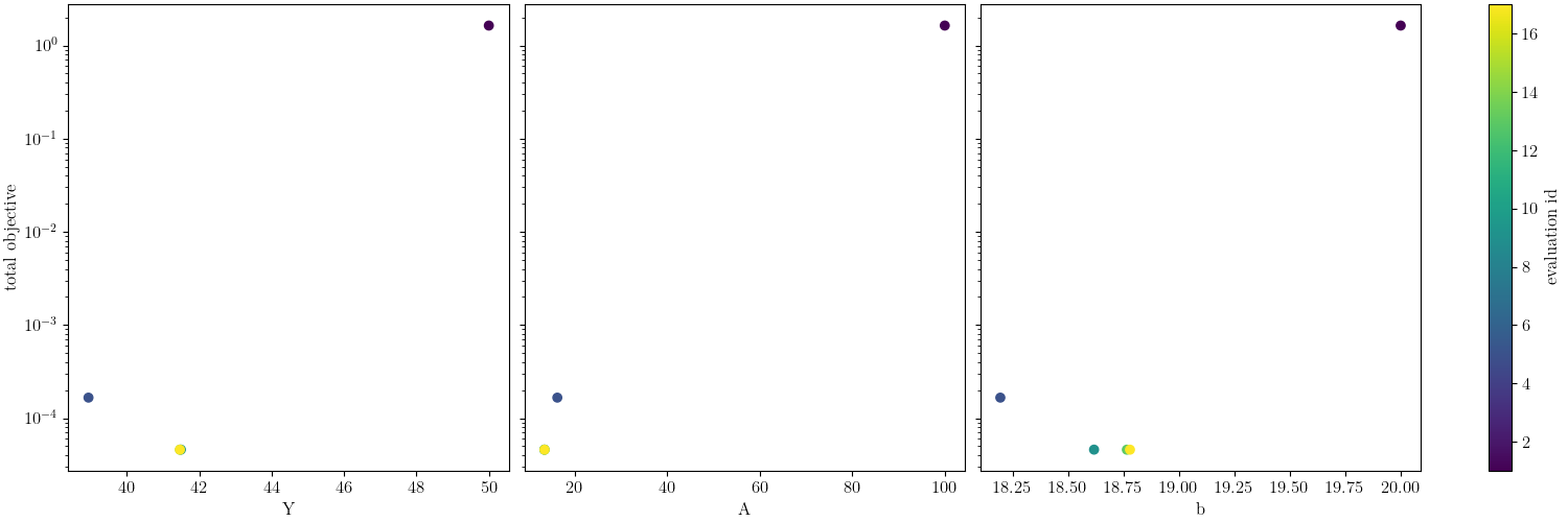
OrderedDict({'Y': 41.467621669, 'A': 13.526784699, 'b': 18.779674534})

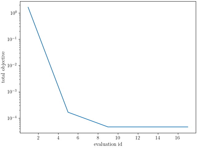
The calibration completes with the Dakota output:

***** RELATIVE FUNCTION CONVERGENCE *****

indicating that the algorithm completed successfully. From the plots it is clear that the model matches the experimental data well, and the final objective function value of around 0.00692 also indicates a quality calibration with low model form error. Since this is a calibration to true stress/strain data, it is also straight forward to verify the fit analytically. From the QoI plot, we can see yield is around 42 ksi and the saturation stress is around 55 ksi which agrees with the calibrated parameters of and .