Uniaxial Loading Material Point Model
MatCal’s UniaxialLoadingMaterialPointModel
is meant to be used in calibrations that can use a material point
model subject to uniaxial loading as the simulation of the experiment.
This can be a valid model for experiments with uniaxial tensile loading without localization
or uniaxial compression experiments without barrelling or buckling. The
UniaxialLoadingMaterialPointModel model has most of the MatCal standard
model features as described in MatCal SIERRA Solid Mechanics Standard Models. Due to
the local nature of the model, only adiabatic thermomechanical loading is supported,
and implicit dynamics is not supported.
In this section, we will provide more information about how the geometry is generated,
specifics on simulation boundary conditions, and what is output from the model.
Note
A suite of examples that include this model can be found at SIERRA/SM Material Point Model Practical Examples
Material point geometry and mesh generation
The MatCal generated material point model is simulated as a unit cube and modeled using a single hexahedral element. No user input parameters are supported or required for geometry generation and discretization.
Uniaxial loading material point boundary conditions
The uniaxial loading material point model has boundary conditions applied in order to load the hexahedral element in a uniaxial stress state. The boundary conditions are shown graphically in Fig. 2.
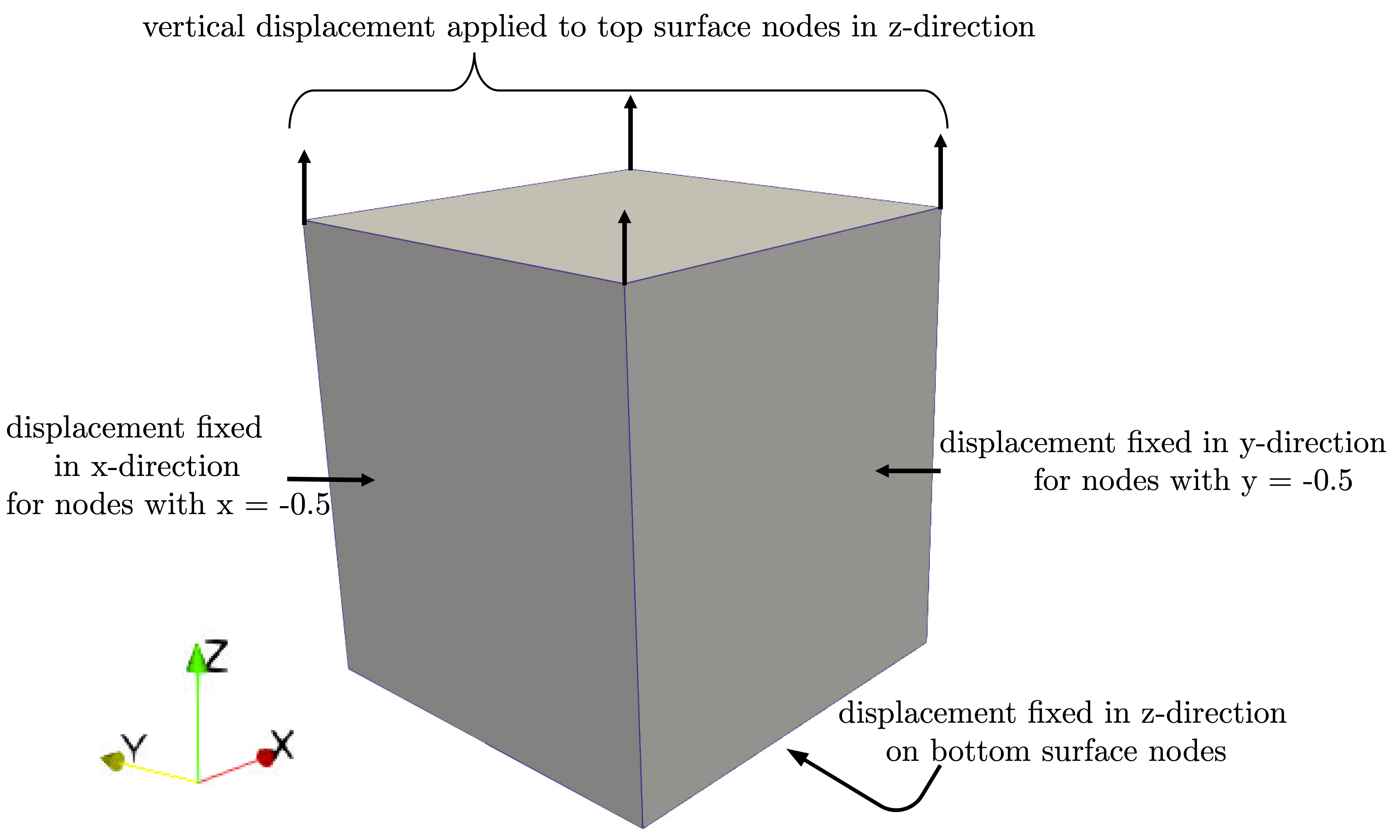
Fig. 2 The single element model and boundary conditions for the uniaxial loading material point model.
In summary, they include:
Displacement boundary conditions on the nodes on two surfaces perpendicular to the loading direction that are fixed in the directions normal to the surfaces on which they are applied.
A displacement boundary condition fixed normal to the loading direction on the nodes on the bottom surface of the element.
An applied displacement function that varies with time to the nodes on the top of the element. The function is determined based on the information in Displacement function determination.
A single node on the bottom surface of the element is fixed in all directions to prohibit rigid body modes.
Displacement function determination
The applied displacement function is calculated for the model based on data supplied to the
add_boundary_condition_data()
method.
This method must be supplied a Data or
DataCollection class that contains
either “engineering_strain” or “true_strain” fields for the
states of interest for the model. They can also optionally include
a “time” field. The
add_boundary_condition_data()
method determines the boundary condition function to be applied
to the model according to the following
algorithm:
Determine the boundary condition by state since maximum deformation, material behavior and experiment setup can vary significantly over different states.
For each state, find the data set with the largest strain and use it for boundary condition generation.
If engineering strain data is provided, select it for the boundary condition generation and ignore true strain data. Since the mesh is a unit cube, the engineering strain can be applied directly to the model as a displacement boundary condition to achieve the correct final deformation.
If engineering strain data is not provided, convert the true strain data to engineering strain and apply this as the displacement boundary condition function.
If the data does not contain a “time” field and there is not a
Stateparameter named “engineering_strain_rate”, then apply a linear displacement function from zero to the maximum engineering strain found in the data over one second.If the data does not contain a “time” field and there is a
Stateparameter named “engineering_strain_rate”, then apply a linear displacement function from zero to the maximum engineering strain found in the data. This is done over a time period beginning at zero seconds and ending at a time calculated by dividing the maximum engineering strain by the “engineering_strain_rate”Stateparameter.If the data does contain a “time” field, use the function directly as provided for the “engineering_strain” field or the engineering strain calculated from the “true_strain” field if no “engineering_strain” field is provided.
Note
Cyclical loading can be modeled with the uniaxial loading
material point model by supplying strain/time data to the
add_boundary_condition_data()
method. This can be useful when modeling stress relaxation and reloading, or
hysteresis. Note that when using the CurveBasedInterpolatedObjective
for complex loading cycles, you may need to use “time” as the independent
variable and “engineering_stress” or “true_stress” as the dependent variables because
it requires monotonically increasing independent variables for interpolation.
Warning
The uniaxial material point model requires that stress and strain values be negative for compression tests and positive for tension tests. Not abiding by this general rule may result in invalid studies even if the models run and studies complete.
Material point thermal model boundary conditions
For a material point,
only adiabatic heating is supported using the
activate_thermal_coupling() method.
When using adiabatic heating, the entire body
of the model is prescribed an initial temperate of
State parameter
“temperature”. For uncoupled simulations, the model is given a prescribed
temperature of State parameter
“temperature” if provided.
Material point model specific output
By default, the material point model includes the following global output fields:
time
displacement - measured in the loading direction at the nodes with the applied displacement function
load - measured at the applied boundary condition nodes in the loading direction.
engineering_strain - same as displacement
engineering_stress - same as load
true_strain - the log strain of the element in the loading direction
true_stress - the Cauchy stress of the element in the loading direction
temperature - the element temperature
contraction - the engineering strain in the x-direction.
log_strain_xx/yy - the log strain of the element in the directions normal to the loading direction
cauchy_stress_xx/yy - the Cauchy stress of the element in the directions normal to the loading direction
All element values are output from the average of all values at element integration points. For the uniaxial loading case, these should be equal, but averaging the values simplifies output for the different element types supported by MatCal’s SIERRA/SM generated models.