Note

Go to the end to download the full example code.

304L bar data analysis

In this example, we analyze the tension data for 304L at several strain rates from [12]. Since 304L material is known to exhibit rate dependence that is measurable when increasing strain rates an order of magnitude or more, this data set is a good data set to analyze for rate dependence. After analyzing the data, we will then use MatCal tools to help chose a model for for the rate dependence.

Note

Useful Documentation links:

First we import the python libraries we will use. For this example, we will use MatCal, NumPy and Matplotlib.

from matcal import *
import matplotlib.pyplot as plt
import numpy as np

plt.rc('text', usetex=True)
plt.rc('font', family='serif')
plt.rc('font', size=12)
figsize = (4,3)

Next, we import the data using the BatchDataImporter. These files have been preprocessed to include state information in each file, so that they can be imported with engineering_strain_rate and temperature state variables pre-assigned to each experiment.

data = BatchDataImporter("ductile_failure_small_tension_data/*.csv").batch

Now that the data is imported, we create data structures that will aid in plotting the yield stresses and stresses at 5 percent strain as a function of rate. We look at these stresses to determine if both yield and hardening are rate dependent. So for each experiment in the data set, we save these values in our data structures. MatCal’s determine_pt2_offset_yield() function is useful here for extracting the 0.2% offset yield stress from engineering stress strain curves.

yield_stresses = {0.0001:[],
                  0.01:[],
                  500.0:[],
                  1800.0:[],
                  3600.0:[]}
five_percent_strain_stresses = {0.0001:[],
                  0.01:[],
                  500.0:[],
                  1800.0:[],
                  3600.0:[]}

for state, data_sets in data.items():
    for data in data_sets:
        rate = state["engineering_strain_rate"]
        yield_pt = determine_pt2_offset_yield(data, 29e3)
        yield_stresses[rate].append(yield_pt[1])
        five_strain = np.interp(0.05, data["engineering_strain"],
                                data["engineering_stress"])
        five_percent_strain_stresses[rate].append(five_strain)

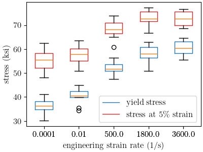
With the data organized as needed, we can create box blots of these values at each rate. This will allow us to see how these values change for each of the measured rates.

plt.figure(figsize=figsize, constrained_layout=True)
bp_yield=plt.boxplot(yield_stresses.values(), labels=yield_stresses.keys())
plt.setp(bp_yield['boxes'], color='tab:blue')
plt.xlabel("engineering strain rate (1/s)")
plt.ylabel("stress (ksi)")
bp_5 =plt.boxplot(five_percent_strain_stresses.values(),
            labels=five_percent_strain_stresses.keys())
plt.setp(bp_5['boxes'], color='tab:red')
plt.legend([bp_yield["boxes"][0], bp_5["boxes"][0]], ['yield stress',
                                                      'stress at 5\% strain'])

/gpfs/knkarls/projects/matcal-stable/external_matcal/documentation/advanced_examples/304L_viscoplastic_calibration/plot_304L_a_data_analysis.py:83: SyntaxWarning: invalid escape sequence '\%'
  'stress at 5\% strain'])

<matplotlib.legend.Legend object at 0x155516cfdaf0>

From these plots, we can see that the material does exhibit rate dependence when the engineering strain rate changes several orders of magnitude. Rate dependence in the material yield is clear. The stresses at five percent strain show that the material hardening is likely rate independent. This is apparent because the stress increase at the different rates does not increase at the stress at 5% strain as would be expected if the material hardening was also rate dependent. Instead it decreases. This decrease is likely due to heating due to plastic work in the material at high rate.

We now plot just the yield data on a semilogx plot to visually assess the relationship between yield stress and strain rate. Two commonly used strain rate dependent yield models for metals include the Johnson-Cook model (JC) and the Power-law Breakdown model (PLB). The functional form for the JC rate dependence model is:

$Y\left(\dot{\epsilon}^p\right) = Y_0\left[1+C\ln\left(\frac{\dot{\epsilon}^p} {\dot{\epsilon}_0}\right)\right]$

where $Y_0$ is the rate independent yield stress, $C$ is a calibration constant, $\dot{\epsilon}^p$ is the material plastic strain rate, and $\dot{\epsilon}_0$ is a reference strain rate under which the material is rate independent. The functional form for the PLB rate dependence model is:

$Y\left(\dot{\epsilon}^p\right) = Y_0\left[1+\text{sinh}^{-1}\left(\left( \frac{\dot{\epsilon}^p}{g}\right)^{(1/m)}\right)\right]$

where $Y_0$ is the rate independent yield stress, and $g$ and $b$ are a calibration constants.

As a function of strain rate, the JC model is linear in a semilogx plot while the PLB can exhibit curvature. To see how these data looks and if one of these model are clearly more appropriate, we plot the data on a semilogx First we put the data into a MatCal matcal.core.data.Data class.

yield_dc = DataCollection("yeild vs rate")
for rate in yield_stresses:
    rate_state = State(f"rate_{rate}", rate=rate)
    for yield_stress in yield_stresses[rate]:
        data = convert_dictionary_to_data({"yield":[yield_stress]})
        data.set_state(rate_state)
        yield_dc.add(data)

Next, we plot the data.

plt.figure(figsize=figsize, constrained_layout=True)
def plot_dc_by_state(data_collection, label=None, color=None, best_index=None):
    for state in data_collection:
        if best_index is None:
            for idx, data in enumerate(data_collection[state]):
                plt.semilogx(state["rate"], data["yield"][0],
                            marker='o', label=label, color=color)
                if color is not None and label is not None:
                    label = "_"+label
        else:
            data = data_collection[state][best_index]
            plt.semilogx(state["rate"], data["yield"][0],
                            marker='o', label=label, color=color)
            if color is not None and label is not None:
                label = "_"+label

    plt.xlabel("engineering strain rate (1/s)")
    plt.ylabel("yield stress (ksi)")
plot_dc_by_state(yield_dc)
plt.show()

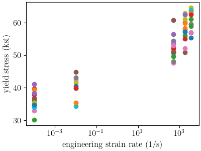
Upon inspection, it is not immediately clear which model will fit the data better. This is likely due to the fact that there is significant scatter at the different strain rates and there is no data in the intermediate strain rates. As a result, we will use MatCal tools to help decide which model we should choose based on these data.

To begin, we calibrate each python model to these data. We already have our data, so we need to create models that can predict the trend in the data. We use MatCal’s PythonModel to implement the models using python functions. These two models are defined below.

First, we define the JC model python function.

def jc_rate_dependence_model(Y_0, C, ref_strain_rate, rate):
    yield_stresses = np.atleast_1d(Y_0*(1+C*np.log(rate/ref_strain_rate)))
    yield_stresses[np.atleast_1d(rate) < ref_strain_rate] = Y_0
    return {"yield":yield_stresses}

Then we create the python model, name it and add the reference strain rate in as a state parameter as it will be uncalibrated.

jc_rate_model = PythonModel(jc_rate_dependence_model)
jc_rate_model.set_name("python_jc_rate_model")
jc_rate_model.add_constants(ref_strain_rate=1e-5)

Next we define the PLB model.

def plb_rate_dependence_model(Y_0, g_star, m, rate):
    yield_stress = Y_0*(1+np.arcsinh((rate/10**(g_star))**(1/m)))
    return {"yield":np.atleast_1d(yield_stress)}

Note that we are calibrating the constant $g$ on a log scale. We create a parameter $g^*$ , such that $g=10^{g*}$ . This is needed because the model would otherwise appear insensitive to $g$ in MatCal studies.

With the function created, we now make the model and name it.

plb_rate_model = PythonModel(plb_rate_dependence_model)
plb_rate_model.set_name("python_plb_rate_model")

Next, we now define the parameters that will be calibrated for these model. Both models will need to calibrate the rate independent yield stress, $Y_0$ . The bounds for this parameter are set based on what we observe in the low strain rate data.

Y_0 = Parameter("Y_0", 20, 60)

The PLB model requires the two parameters $g_star$ and $m$ . The $g$ parameter is meant to represent a change in behavior for the rate dependence. It is based on experimental observations that show materials sensitivity to rate increase at high strain rates. In this model, it can be considered a reference rate above which the material becomes more rate sensitive. Since this is generally at higher rates for metals, we restrict this reference rate to be between 100 and 10000 per second. Any lower or higher, and the parameter will be used in an unintended fashion. The bounds for $m$ are set based on our previous experience with the model for austenitic stainless steels.

g_star = Parameter("g_star", 2, 4)
m = Parameter("m", 2, 15)

The only unique parameter for the JC model is the calibration parameter $C$ which we also set bounds for using our previous experience with the model for metals.

C = Parameter("C", 0.001, 0.1)

The last component needed for our calibrations is the objective. We use a Objective to fit our python models to the data.

obj = Objective("yield")

Now we can setup our calibrations and save the results.

jc_cal = GradientCalibrationStudy(Y_0, C)
jc_cal.add_evaluation_set(jc_rate_model, obj, yield_dc)
jc_cal.set_working_directory("jc", remove_existing=True)
jc_cal_results = jc_cal.launch()

plb_cal = GradientCalibrationStudy(Y_0, g_star, m)
plb_cal.add_evaluation_set(plb_rate_model, obj, yield_dc)
plb_cal.set_working_directory("plb", remove_existing=True)
plb_cal_results = plb_cal.launch()

With the calibrations complete, we plot the fits against the data and print the best fit information.

jc_best_idx = jc_cal_results.best_evaluation_index
jc_best_sim = jc_cal_results.simulation_history[jc_rate_model.name]

plb_best_idx = plb_cal_results.best_evaluation_index
plb_best_sim = plb_cal_results.simulation_history[plb_rate_model.name]

plt.figure(figsize=figsize, constrained_layout=True)
plot_dc_by_state(yield_dc, "experiments" , 'k')
rates=np.logspace(-4,4,100)
plt.semilogx(rates, jc_rate_dependence_model(**jc_cal_results.best.to_dict(),
                                             ref_strain_rate=1e-5,
                                             rate=rates)['yield'], label="JC model")
plot_dc_by_state(jc_best_sim, None, 'tab:blue', best_index=jc_best_idx)
plt.semilogx(rates, plb_rate_dependence_model(**plb_cal_results.best.to_dict(),
                                             rate=rates)['yield'], label="PLB model")
plot_dc_by_state(plb_best_sim, None, 'tab:orange', best_index=plb_best_idx)
plt.legend()
plt.show()

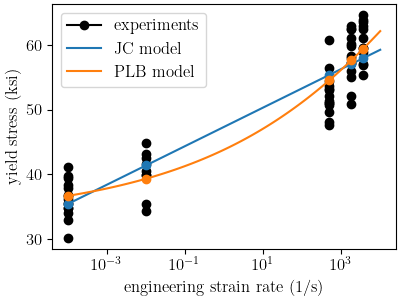
From this plot, both models appear to represent the data well. Looking at the final total objective and parameters will reveal which model fits the data better and if there were any issues in the fitting process.

jc_eval_set_name = f"{jc_rate_model.name}:{obj.name}"
jc_best_obj = jc_cal_results.best_total_objective
print("JC model best fit objective:", jc_best_obj)
print(jc_cal_results.best.to_dict(),"\n")

plb_eval_set_name = f"{plb_rate_model.name}:{obj.name}"
plb_best_obj = plb_cal_results.best_total_objective
print("PLB model best fit objective:", plb_best_obj)
print(plb_cal_results.best.to_dict(),"\n")

JC model best fit objective: 0.004652787936813707
OrderedDict({'Y_0': 32.444999516, 'C': 0.039894200734})

PLB model best fit objective: 0.004014596531156934
OrderedDict({'Y_0': 33.037043219, 'g_star': 4.0, 'm': 8.3580048779})

The objectives show that the PLB model provides a better fit to these data. However, we can see in the fit that its parameter for $g_star$ is hitting its upper bound. This is showing that the calibration is adjusting that parameter outside is intended use case for this model and is the first indication that we should use JC over PLB.

To look into this further, we will perform a sensitivity study on the objective with respect to the parameters in both models. If the objective is not very sensitive to the parameters, it can be an indication that the parameter is not very well defined by the given objective.

We start with the JC model. We need to redefine our parameters and add distributions to them to support the sensitivity study. We will assign them a uniform_uncertain distribution.

Y_0 = Parameter("Y_0", 20, 60, distribution="uniform_uncertain")
C = Parameter("C", 0.001, 0.1, distribution="uniform_uncertain")

Now we can create our LhsSensitivityStudy and add our evaluation set.

Note

We update the metric function of the objective to be the L2NormMetricFunction. This can provide a more interpretable result for sensitivity analyses than the SumSquaresMetricFunction.

sens = LhsSensitivityStudy(Y_0, C)
obj.set_metric_function(L2NormMetricFunction())
sens.add_evaluation_set(jc_rate_model, obj, yield_dc)
sens.set_working_directory("jc_sens", remove_existing=True)

We want to perform the study on the overall objective and to perform a Sobol index study. The Sobol index study provides a global sensitivity of the models to the input parameters and are valid for nonlinear responses.

sens.use_overall_objective()
sens.make_sobol_index_study()

Since the python model is inexpensive, we take 2500 samples. For a problem with a more computationally expensive model, you should run many studies with increasing samples until the Sobol indices converge.

num_samples = 2500
sens.set_number_of_samples(num_samples)

For python models, performance gains can be achieved by running the evaluations in serial. Parallel evaluations require additional overhead that can decrease performance when using inexpensive models such as a PythonModel.

sens.run_in_serial()

We now launch the study and save the results.

jc_sens_results = sens.launch()

The sensitivity study for the PLB model is setup the same way.

g_star = Parameter("g_star", 2, 4,distribution="uniform_uncertain")
m = Parameter("m", 2, 15, distribution="uniform_uncertain")

sens = LhsSensitivityStudy(Y_0, g_star, m)
sens.add_evaluation_set(plb_rate_model, obj, yield_dc)
sens.set_number_of_samples(num_samples)
sens.set_working_directory("plb_sens", remove_existing=True)
sens.use_overall_objective()
sens.make_sobol_index_study()
sens.run_in_serial()

We once again launch the study and save the results.

plb_sens_results = sens.launch()

With both studies complete, we can print the results for analysis.

print("JC sensitivity results:", jc_sens_results.sobol)
print("PLB sensitivity results:", plb_sens_results.sobol)

JC sensitivity results: Y_0: [[0.48219582 0.7043585 ]]
C: [[0.25280175 0.49818737]]
PLB sensitivity results: Y_0: [[0.85005052 0.91571222]]
g_star: [[0.02345957 0.10134016]]
m: [[0.00910786 0.04080117]]

The results are printed for each parameter and show the main effects and total effects, respectively. These responses show that the JC model should be used since both its parameters have significant main and total effects. With main effects of ~> 0.3 and total effects ~> 0.6, Both $Y_0$ and $C$ have a measurable influence on the objective and are significantly coupled. While for the PLB model, $m$ and $g_star$ only have a slight influence on the objective with main effects < 0.1. Even the total effect of $m$ is < 0.1. This indicates they cannot be well calibrated over their expected ranges with the available data and this model should not be used.

To finish this study, we save the JC calibrated parameters and the yield vs rate data to a file for use in the full finite element calibration.

matcal_save("JC_parameters.serialized", jc_cal_results.best.to_dict())
matcal_save("rate_data.joblib", yield_dc)

Total running time of the script: (35 minutes 22.710 seconds)

Gallery generated by Sphinx-Gallery