Parameter uncertainty example - external noise and internal variability

Once again, for this example, the data comes from the same model as the one we are calibrating. It is similar to the Data Noise Issue - Low and High Noise Example, but demonstrates the two different Laplace approximation methods available in MatCal.

The model is a bilinear function similar to elastic-plastic response with the parameter “Y” controlling where change from one linear trend to the other takes place and the parameter “H” controlling the slope of the second trend. The slope of the initial trend is fixed, as if it were known (as the elastic modulus typically would be). The problem differs from the referenced example when we generate the data for the model. We will use the model to generate data with uncertainty from two sources: noise and parameter uncertainty.

from matcal import *
import numpy as np

After importing the tools from MatCal, we create the model for this example. We will use a PythonModel and define the python function that will be the underlying code driving the model. The data will be fitted to a model with a bilinear response similar to an elastic-plastic model. The initial slope (E) is assumed to be known. The parameter “Y” determines where the model changes to the second linear trend The parameter “H” determines the second slope.

def bilinear_model(**parameters):
  max_strain = 1.0
  npoints = 100
  strain = np.linspace(0,max_strain,npoints)
  E = 1.5
  Y = parameters['Y']
  H = parameters['H']
  eY = Y/E
  stress = np.where(strain < eY, E*strain, Y + H*(strain-eY))
  response = {'strain':strain, 'stress': stress}
  return response

With the function defined, we can now create the MatCal model and study parameters.

model = PythonModel(bilinear_model)
model.set_name("bilinear")
Y = Parameter('Y',0.0,1.0, 0.501)
H = Parameter('H',0.0,1.0, 0.501)
parameters = ParameterCollection('parameters', Y, H)

We then use the model function directly to generate our data for the study. As previously stated, we generate data that has both: (a) external “measurement” noise and (b) variability in the underlying response e.g. due to different processing of the same material. In order to do so we need to import some more tools to support our random number generation and create a DataCollection with our generated data.

import copy
from numpy.random import default_rng
_rng = default_rng(seed=1234)

exp_stddev = 0.005
parameter_mean = [0.15,0.1]
parameter_covariance = [[0.00005,0.0],[0.0,0.00005]]

generation for a given number of samples and generate data for a low number of samples as is typical with real experimental data. We will repeat this later for more samples to show the matcal.core.parameter_studies.LaplaceStudy converges to the truth parameter covariance as the number of samples increases.

def generate_data(n_samples):
    data = DataCollection("noisy_data")
    parameter_samples = _rng.multivariate_normal(parameter_mean,
                                                 parameter_covariance,n_samples)
    for p in parameter_samples:
        p_dict = {'Y':p[0],'H':p[1]}
        response = bilinear_model(**p_dict)
        d = copy.deepcopy(response)

        d["stress"] += exp_stddev*_rng.standard_normal(len(d["stress"]))
        data.add(convert_dictionary_to_data(d))
    return data
data = generate_data(5)

Next, we start with finding the least squares best fit parameters with gradient-based calibration. We create the calibration for our model parameters, and define an objective for fitting the model response to the data. Once again, we put this in a function so that it can be re-used later.

objective = CurveBasedInterpolatedObjective('strain','stress')
objective.set_name("objective")
def get_best_fit(data):
    calibration = GradientCalibrationStudy(parameters)
    calibration.add_evaluation_set(model, objective, data)
    results = calibration.launch()
    return results

Then we run the calibration and store the results.

results = get_best_fit(data)

After running the calibration, we load the optimal parameters and the best fit mode response. Note the best parameters are close but not precisely the mean parameters used to generate the data.

state_name = data.state_names[0]
best_parameters = results.best.to_dict()
best_response = results.best_simulation_data(model.name, state_name)

print("Best fit parameters:")
print(results.best)

Best fit parameters:
Y: 0.14494742222
H: 0.10829321178

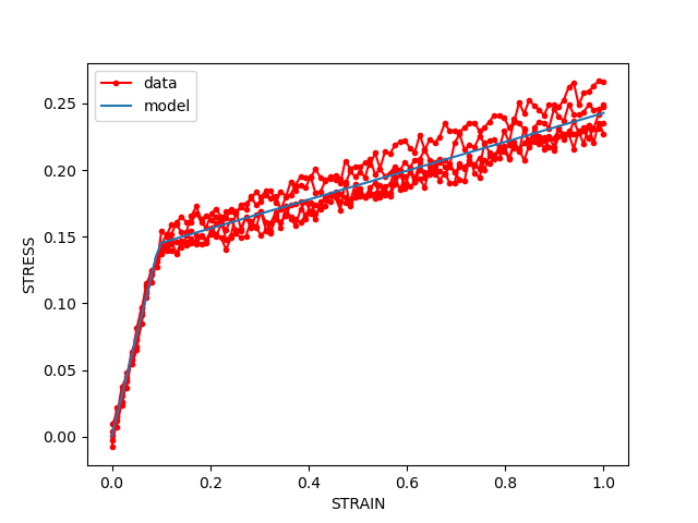
Now compare the model (lines) response to the data (red lines with points). In the eyeball norm the best fit model is in the middle of the noisy data, i.e. there are about as many points above the fitted line as below. This is due to using a mean squared error objective.

import matplotlib.pyplot as plt
def compare_data_and_model(data,model_response,fig_label=""):
  for c in data.values():
    for i,d in enumerate(c):
      d = convert_data_to_dictionary(d)
      plt.figure(fig_label)
      label = None
      if i==0:
        label = "data"
      plt.plot(d['strain'],d['stress'],'-ro',ms=3,label=label)
  for i,response in enumerate(model_response):
    plt.figure(fig_label)
    label = None
    if i==0:
      label="model"
    plt.plot(response['strain'], response['stress'], label=label)

  plt.figure(fig_label)
  plt.xlabel("STRAIN")
  plt.ylabel("STRESS")
  plt.legend()
  plt.show()

compare_data_and_model(data,[best_response],fig_label="best fit calibration")

Now we investigate the effect of noise on the parameter uncertainty using MatCal’s ClassicLaplaceStudy for (inexpensive, approximate) uncertainty quantification. The LaplaceStudy uses the Laplace approximation to calibrate a mutlivariate normal distribution characterizing the parameter uncertainty. Since it uses the parameter hessian near the optimum parameters it is an approximation of the parameter uncertainty obtained by more expensive methods. We use the same data and give the Laplace study the optimal parameters to use as a center for the finite difference evaluation of the Hessian. After initial setup, we can run the uncertainty quantification studies.

laplace = ClassicLaplaceStudy(parameters)
laplace.add_evaluation_set(model, objective, data)
laplace.set_parameter_center(**best_parameters)
laplace_results_external = laplace.launch()

When they finish, we can sample the resulting distributions using matcal.core.parameter_studies.sample_multivariate_normal(). We request 50 samples.

num_samples = 50
noisy_parameters = sample_multivariate_normal(num_samples, laplace_results_external.mean.to_list(),
                                              laplace_results_external.estimated_parameter_covariance,
                                              param_names=laplace_results_external.parameter_order)

For each sample, we run the parameters through the model using a matcal.core.parameter_studies.ParameterStudy so that we can compare the uncertain model to the data.

def push_forward_parameter_samples(parameters,samples):
  param_study = ParameterStudy(parameters)
  param_study.add_evaluation_set(model, objective, data)
  for Y_samp, H_samp in zip(samples["Y"], samples["H"]):
    param_study.add_parameter_evaluation(Y=Y_samp, H=H_samp)
  results = param_study.launch()
  responses = []
  for i in range(num_samples):
    response = results.simulation_history[model.name][state_name][i]
    responses.append(response)
  return responses
model_response = push_forward_parameter_samples(parameters, noisy_parameters)

Now we plot a comparison of the model responses and the calibration data.

compare_data_and_model(data,model_response,
                       fig_label="model response samples from external noise assumption")

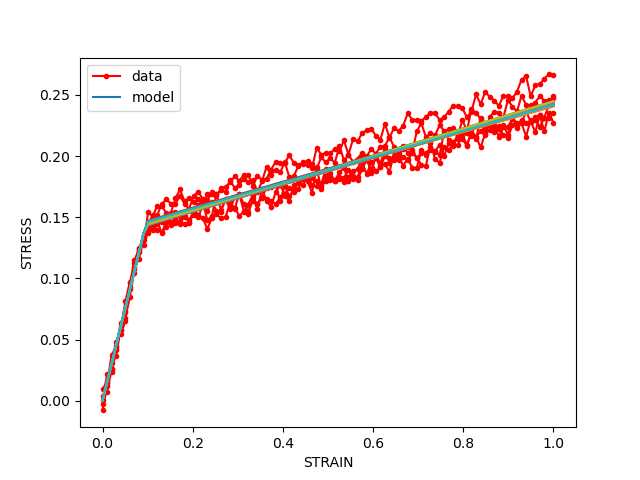
Note how the data is not encapsulated by the estimated uncertainty. This is because there are many points included in the calibration and the uncertainty due to noise is small.

Next We compare the estimated parameter covariance with the known covariance using a percent error measure and see that the error is quite high as expected.

def compare_laplace_results(estimated_covar):
    print("Estimated covariance:")
    print(estimated_covar)
    print("\n")
    print("Actual covariance:")
    print(parameter_covariance)
    print("\n")
    print("% Error:", (np.mean(estimated_covar-parameter_covariance)
                       /np.mean(parameter_covariance)*100))
    print("\n")


compare_laplace_results(laplace_results_external.estimated_parameter_covariance)

Estimated covariance:
[[ 1.13224298e-06 -1.73466023e-06]
 [-1.73466023e-06  3.54597886e-06]]


Actual covariance:
[[5e-05, 0.0], [0.0, 5e-05]]


% Error: -98.791098614358

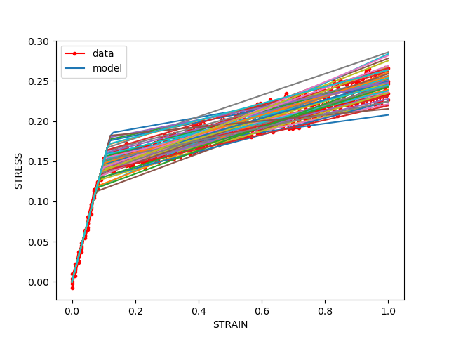
We now examine the parameter distribution when the error is attributed to model form error as is done with the LaplaceStudy Here the variability is associated with variability of the model parameters. For this example the parameter distribution tends to cover the calibration data, but the quality of the estimate is dependent on the number of data samples included and how well the data conform to a multivariate normal. We perform the same plotting and percent error calculation as was done for the .

def estimate_uncertainty_due_model_error(data):
    laplace = LaplaceStudy(parameters)
    laplace.add_evaluation_set(model, objective, data)
    laplace.set_parameter_center(**best_parameters)
    laplace.set_noise_estimate(exp_stddev)
    laplace_results_internal = laplace.launch()
    print("Mean",laplace_results_internal.mean.to_list())
    print("Covar",laplace_results_internal.estimated_parameter_covariance)
    print("Param order", laplace_results_internal.parameter_order)
    uncertain_parameters = sample_multivariate_normal(num_samples,
                                                      laplace_results_internal.mean.to_list(),
                                                      laplace_results_internal.estimated_parameter_covariance,
                                                       param_names=laplace_results_internal.parameter_order)
    model_response = push_forward_parameter_samples(parameters, uncertain_parameters)
    compare_data_and_model(data,model_response,fig_label="model response samples from internal variability assumption")
    compare_laplace_results(laplace_results_internal.estimated_parameter_covariance)

estimate_uncertainty_due_model_error(data)

Mean [0.14494742222, 0.10829321178]
Covar [[ 0.00025919 -0.00027995]
 [-0.00027995  0.00067829]]
Param order ['Y', 'H']
Estimated covariance:
[[ 0.00025919 -0.00027995]
 [-0.00027995  0.00067829]]


Actual covariance:
[[5e-05, 0.0], [0.0, 5e-05]]


% Error: 277.5792961717505

Note how the data is now encapsulated by the estimated uncertainty. This is because the error is now appropriately attributed to uncertainty in the model. Also, the estimate for the parameter covariance has improved, although it is still higher than we would like for verification.

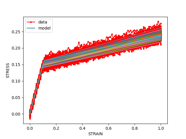
Next, we redo the study with more sample and see the effect it has on the predicted parameter uncertainty..

data = generate_data(200)
results = get_best_fit(data)
best_parameters = results.best.to_dict()
estimate_uncertainty_due_model_error(data)

Mean [0.15019281551, 0.099968038367]
Covar [[ 5.16138267e-05 -3.62031219e-06]
 [-3.62031219e-06  5.92064747e-05]]
Param order ['Y', 'H']
Estimated covariance:
[[ 5.16138267e-05 -3.62031219e-06]
 [-3.62031219e-06  5.92064747e-05]]


Actual covariance:
[[5e-05, 0.0], [0.0, 5e-05]]


% Error: 3.5796769584691197

The 50 samples propagated through the model have less spread. This is because the uncertainty attributed to parameter uncertainty is better accounted for with the larger sample size. Also, the percent error metric is much improved showing that the result is approaching the expected value.