Calibration of Two Different Material Conductivities

In this section, we will cover how to run a calibration study using a model for an external physics modeling software. Specifically, we will be calibrating the conductivities of a layered material consisting of a layer of stainless steel and a layer of ceramic foam. We have experimental data from thermocouples placed on the free-surface of the stainless steel layer and at the steel-foam interface while the ceramic was subjected to a steady heat flux. We obtain temperature versus time data from the experiments run at different applied heat fluxes. We have preprocessed the data file by removing any errant lines and truncating the data set to the times relevant to the experiment. The preprocessed data is stored in csv files named ‘layered_heat_test_high_0.csv’, ‘layered_heat_test_high_1.csv’, and ‘layered_heat_test_low.csv’. We have two data sets run in the high flux configuration, and one data set from the low flux configuration.

MatCal has no native ability to perform physics calculations, therefore, this needs to be done by an outside program. For this case we use the Sandia thermal-fluids code SIERRA/Aria. Prior to running this calibration, we created and tested a SIERRA/Aria input file and mesh file that represents our experimental configuration. The SIERRA/Aria input file is named ‘two_material_square.i’ and the mesh file is named ‘two_material_square.g’. After creating these files, we prepare them for use in MatCal.

Preprocessing Sierra Input Files

In order for MatCal to safely pass a set of parameters to evaluate into our model, it uses Aprepro to annotate the variable values at the top of the input files we provide to it. To prepare our files, we replace our tentative parameter values in our material models with variable aliases in the Aprepro style curly brackets. For instance we take the following line:

conductivity = constant value = 1

and replace it with:

conductivity = constant value = {K_foam}

K_foam will be the name we assign to a parameter in our study. In addition to replacing the material parameters we wish to calibrate, we need to also have a variable alias that relates to our different boundary heat fluxes. For Aria, we can do this by adding the alias in the boundary condition specification:

BC Flux for energy on surface near_heater_surface = constant value = {exp_flux}

We will use the variable alias exp_flux to make sure our model is run under the same state conditions as our experimental data was gathered in. Now that these steps are complete, we can start writing our MatCal script.

We start off our script as we have in the previous examples; importing MatCal and defining the parameters we wish to study.

Note

As a reminder, the names we give our parameters (K_foam, K_steel) need to be the same names used in our input file.

from matcal import *

cond_1 = Parameter("K_foam", .05 , .5, distribution="uniform_uncertain")
cond_2 = Parameter("K_steel", 40, 50, distribution="uniform_uncertain")

The next step is to import our cleaned experimental data. We have data from two different heat flux rates. In order for MatCal to compare the correct experimental data to the correct simulation results, each of the data sets imported need to have a State assigned to them. Below we import the low heat flux data.

low_flux_data = FileData("layered_heat_test_low.csv")

low_flux_state = State("LowFlux", exp_flux=1e3)
low_flux_data.set_state(low_flux_state)

First, we import the data as we have in previous examples. Then, we create a state and assign it to our data using the set_state() method. Passing data with states into a MatCal study will let MatCal know that it needs to run a particular simulation multiple times in each of the different experimental states. This way we only need to supply one input deck for a given experimental setup no matter the number of different variables changed between runs.

If we were running a Python model, the state parameters would be passed into the Python function along with the study parameters as keyword arguments, so that both the state and study parameters are accessible in the model.

A state is created using a State object. A State object takes in a name for the state, in this case ‘LowFlux’, and then keyword arguments for the variables that describe that state. In this case we have one variable exp_flux, which tells our input file how much heat to impose on our target surface.

We then repeat this process for the high heat flux data.

high_flux_state = State("HighFlux", exp_flux=1e4)
high_flux_data_0 = FileData("layered_heat_test_high_0.csv")
high_flux_data_1 = FileData("layered_heat_test_high_1.csv")

high_flux_data_0.set_state(high_flux_state)
high_flux_data_1.set_state(high_flux_state)

The two high heat flux datasets are run with the same flux, so they share the same state. In MatCal, all states should be unique, and a single state can be assigned to multiple datasets. While we wrote our data importing explicitly in this example, if we had more repeats of our experiments, it would be easier for us to import data using the BatchDataImporter. See Data Importing and Manipulation.

With our individual pieces of data imported, we then group it all together in a DataCollection, which is a cohesive set of data that can be used together to calibrate a given model.

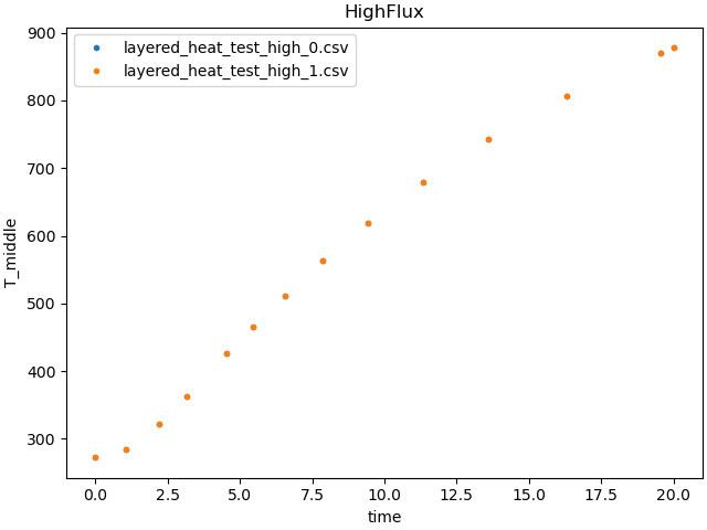
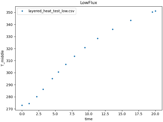
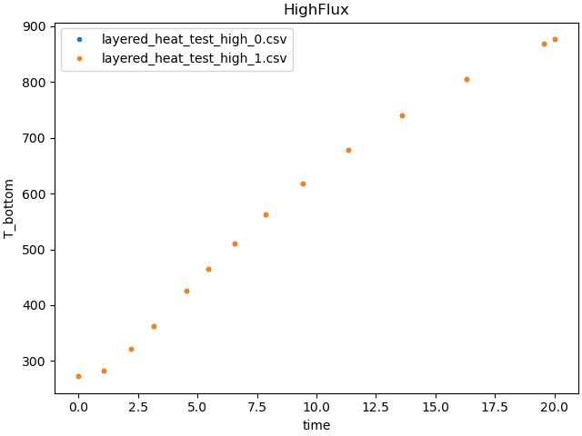
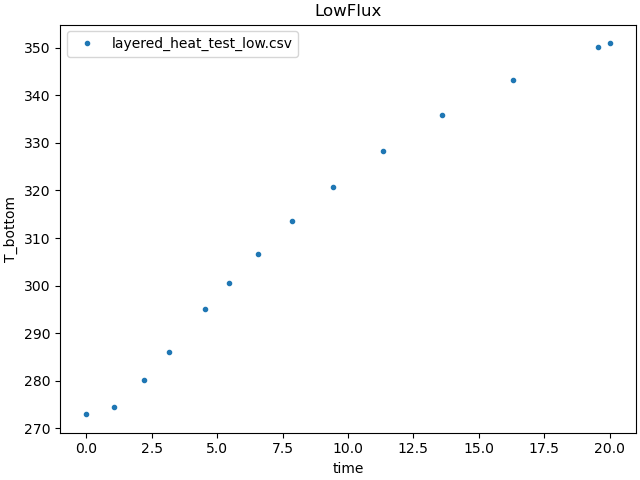
data_collection = DataCollection("temperature_data", high_flux_data_0, high_flux_data_1, low_flux_data)
data_collection.plot("time", "T_middle")
data_collection.plot("time", "T_bottom")

• 
• 
• 
• 

Now we define that model for MatCal.

user_file = "two_material_square.i"
geo_file = "two_material_square.g"
sim_results_file = "two_material_results.csv"
model = UserDefinedSierraModel('aria', user_file, geo_file)

SIERRA models that we create on our own are imported into MatCal using the UserDefinedSierraModel class. The first argument we pass in is the name of the SIERRA executable we wish to run, in our case aria to run SIERRA/Aria. The second and third arguments are the file paths to the input file and mesh file, respectively. MatCal expects that the simulation will import the mesh file from the current working directory when it is run. As a result, MatCal might run into errors if the mesh file and input file are supplied in different directories. If there are any additional files or directories needed to to run the model, we could just add their filepaths as additional arguments after the mesh file.

The last thing we need is to tell MatCal what results csv file our Aria simulation will produce. MatCal by default expects ‘results.csv’ to be the results file produced by any model, and since ours has a different name, we need to provide this to MatCal.

model.set_results_filename(sim_results_file)

# Now that we have our model and data setup,
# we setup and run our calibration study just like our previous examples.

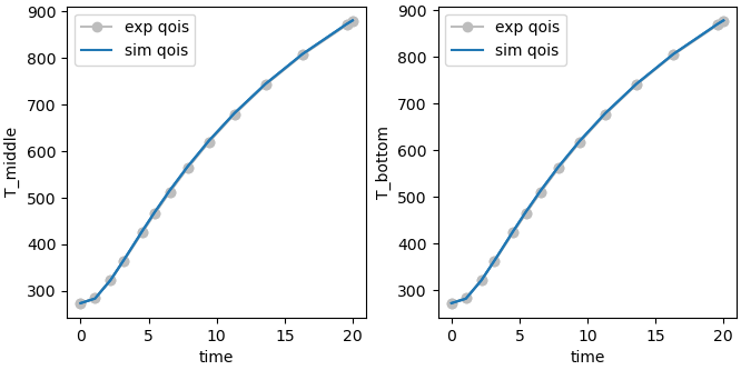
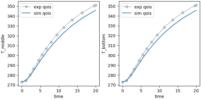
objective = CurveBasedInterpolatedObjective("time", "T_middle", "T_bottom")

We define an objective to compare the data fields “T_middle” and “T_bottom” across “time” for our experimental data and simulation data.

calibration = GradientCalibrationStudy(cond_1, cond_2)
calibration.set_results_storage_options(results_save_frequency=3)
calibration.add_evaluation_set(model, objective, data_collection)
calibration.set_core_limit(6)

We define our calibration study, telling it what parameters we are studying. We then assign an evaluation set to the study, telling the study that it compares a given set of data, to the given model, in the way described by the given objective. Lastly, we let the study know how many cores it can use.

With the calibration setup, all that is left to do is run it, wait for the results and plot the completed calibration results.

results = calibration.launch()
print(results.best.to_dict())
make_standard_plots("time")

• 
• 
• 
• 

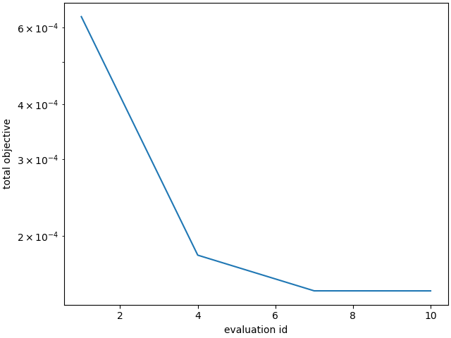
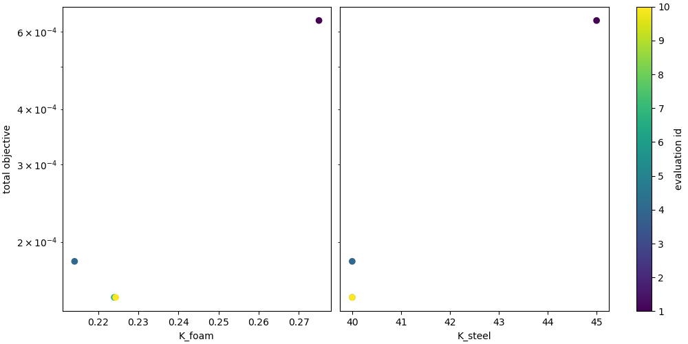
OrderedDict({'K_foam': 0.2243968746, 'K_steel': 40.0})