Note
Go to the end to download the full example code.
304L stainless steel viscoplastic calibration uncertainty quantification
In this example, we will use MatCal’s LaplaceStudy
to estimate the parameter uncertainty for the calibration.
Warning
The LaplaceStudy is still in development and may not accurately attribute uncertainty to to the parameters. Always verify results before use.
To begin, we once again reuse the data import, model preparation and objective specification for the tension model and rate models from the original calibration.
import numpy as np
import matplotlib.pyplot as plt
from matcal import *

plt.rc('text', usetex=True)
plt.rc('font', family='serif')
plt.rc('font', size=12)
figsize = (4,3)

tension_data = BatchDataImporter("ductile_failure_ASTME8_304L_data/*.dat",
                                    file_type="csv")
tension_data.set_fixed_state_parameters(displacement_rate=2e-4, temperature=530)
tension_data = tension_data.batch
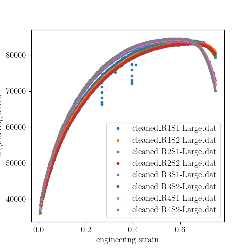
We then manipulate the data to fit our needs and modeling choices. First, we scale the data from ksi to psi units. Then we remove the time field as this has consequences for the finite element model boundary conditions. See Uniaxial tension solid mechanics boundary conditions.
tension_data = scale_data_collection(tension_data, "engineering_stress", 1000)
tension_data.remove_field("time")

down_selected_data = DataCollection("down selected data")
for state in tension_data.keys():
   for index, data in enumerate(tension_data[state]):
      down_selected_data.add(data[(data["engineering_stress"] > 36000) &
                                  (data["engineering_strain"] < 0.75)])
Next, we plot the data to verify we imported the data as expected.
astme8_fig = plt.figure(figsize=(5,5))
down_selected_data.plot("engineering_strain", "engineering_stress",
                    figure=astme8_fig)
/gpfs/knkarls/projects/matcal_devel/external_matcal/matcal/core/data.py:588: UserWarning: Ignoring specified arguments in this call because figure with num: 1 already exists
  plt.figure(figure.number, constrained_layout=True)
We also import the rate data as we will need to recalibrate
the Johnson-Cook parameter  since
since  will
likely be changing. We put it in a
will
likely be changing. We put it in a DataCollection
to facilitate plotting.
rate_data_collection = matcal_load("rate_data.joblib")
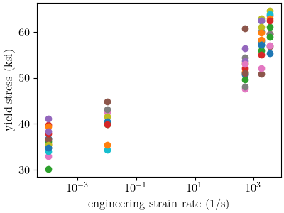
Next, we plot the data on with a semilogx plot to verify it imported
as expected.
plt.figure(figsize=(4,3), constrained_layout=True)
def make_single_plot(data_collection, state, cur_idx, label,
                     color, marker, **kwargs):
    data = data_collection[state][cur_idx]
    plt.semilogx(state["rate"], data["yield"][0],
                marker=marker, label=label, color=color,
                **kwargs)

def plot_dc_by_state(data_collection, label=None, color=None,
                     marker='o', best_index=None, only_label_first=False, **kwargs):
    for state in data_collection:
        if best_index is None:
            for idx, data in enumerate(data_collection[state]):
                make_single_plot(data_collection, state, idx, label,
                                 color, marker, **kwargs)
                if ((color is not None and label is not None) or
                    only_label_first):
                    label = None
        else:
            make_single_plot(data_collection, state, best_index, label,
                             color, marker, **kwargs)
    plt.xlabel("engineering strain rate (1/s)")
    plt.ylabel("yield stress (ksi)")
plot_dc_by_state(rate_data_collection)
plt.show()

calibrated_params = matcal_load("voce_calibration_results.serialized")

Y_0 = Parameter("Y_0", 20, 60,
                calibrated_params["Y_0"])
A = Parameter("A", 100, 400,
              calibrated_params["A"])
b = Parameter("b", 0, 3,
              calibrated_params["b"])
C = Parameter("C", -3, -0.5, calibrated_params["C"])
X = Parameter("X", 0.50, 1.75, 1.0)

def JC_rate_dependence_model(Y_0, A, b, C, X, ref_strain_rate, rate, **kwargs):
    yield_stresses = np.atleast_1d(Y_0*X*(1+10**C*np.log(rate/ref_strain_rate)))
    yield_stresses[np.atleast_1d(rate) < ref_strain_rate] = Y_0
    return {"yield":yield_stresses}

rate_model = PythonModel(JC_rate_dependence_model)
rate_model.set_name("python_rate_model")

material_name = "304L_viscoplastic"
material_filename = "304L_viscoplastic_voce_hardening.inc"
sierra_material = Material(material_name, material_filename,
                            "j2_plasticity")

geo_params = {"extensometer_length": 0.75,
               "gauge_length": 1.25,
               "gauge_radius": 0.125,
               "grip_radius": 0.25,
               "total_length": 4,
               "fillet_radius": 0.188,
               "taper": 0.0015,
               "necking_region":0.375,
               "element_size": 0.01,
               "mesh_method":3,
               "grip_contact_length":1}

astme8_model = RoundUniaxialTensionModel(sierra_material, **geo_params)
astme8_model.add_boundary_condition_data(tension_data)

from site_matcal.sandia.computing_platforms import is_sandia_cluster, get_sandia_computing_platform
from site_matcal.sandia.tests.utilities import MATCAL_WCID

cores_per_node = 24
if is_sandia_cluster():
    platform = get_sandia_computing_platform()
    cores_per_node = platform.processors_per_node

astme8_model.set_number_of_cores(cores_per_node)
if is_sandia_cluster():
    astme8_model.run_in_queue(MATCAL_WCID, 1)
    astme8_model.continue_when_simulation_fails()
astme8_model.set_allowable_load_drop_factor(0.45)
astme8_model.set_name("ASTME8_tension_model")
astme8_model.add_constants(ref_strain_rate=1e-5)

X_calibrated = calibrated_params.pop("X")
rate_model.add_constants(ref_strain_rate=1e-5, X=X_calibrated)
astme8_model.add_constants(ref_strain_rate=1e-5)

rate_objective = Objective("yield")
astme8_objective = CurveBasedInterpolatedObjective("engineering_strain", "engineering_stress")
We can now setup a LaplaceStudy
and add the evaluation sets of interest. We use the default options for the
study as these are the most robust.
See 6061T6 aluminum calibration uncertainty quantification to
see the effect of changing the noise_estimate.
params = ParameterCollection("laplace params", Y_0, A, b, C)
laplace = LaplaceStudy(Y_0, A, b, C)
laplace.add_evaluation_set(astme8_model, astme8_objective, down_selected_data)
laplace.add_evaluation_set(rate_model, rate_objective, rate_data_collection)
laplace.set_core_limit(112)
cal_dir = "laplace_study"
laplace.set_working_directory(cal_dir, remove_existing=True)
We set the parameter center to the calibrated parameter values and launch the study.
laplace.set_parameter_center(**calibrated_params)
laplace_results = laplace.launch()
print("Initial covariance estimate:\n", laplace_results.estimated_parameter_covariance)
print("Calibrated covariance estimate:\n", laplace_results.fitted_parameter_covariance)
matcal_save("laplace_study_covariance.joblib", laplace_results.fitted_parameter_covariance)
Initial covariance estimate:
 [[ 1.32115570e+01  4.61400061e+01 -1.00034011e+00 -1.02329273e+00]
 [ 4.61400061e+01  2.67119860e+02 -5.48852002e+00 -4.06085165e+00]
 [-1.00034011e+00 -5.48852002e+00  1.14461084e-01  8.58810450e-02]
 [-1.02329273e+00 -4.06085165e+00  8.58810450e-02  8.21702040e-02]]
Calibrated covariance estimate:
 [[ 1.32115606e+01  4.61399850e+01 -1.01189534e+00 -1.02329366e+00]
 [ 4.61399850e+01  2.67119452e+02 -5.48851392e+00 -4.09821969e+00]
 [-1.01189534e+00 -5.48851392e+00  1.14461008e-01  8.58810924e-02]
 [-1.02329366e+00 -4.09821969e+00  8.58810924e-02  8.21703308e-02]]
We see that the initial and calibrated covariance estimates are nearly equal. This is because the variance in the data is relatively low and the model form error for the model when compared to the experiments is low.
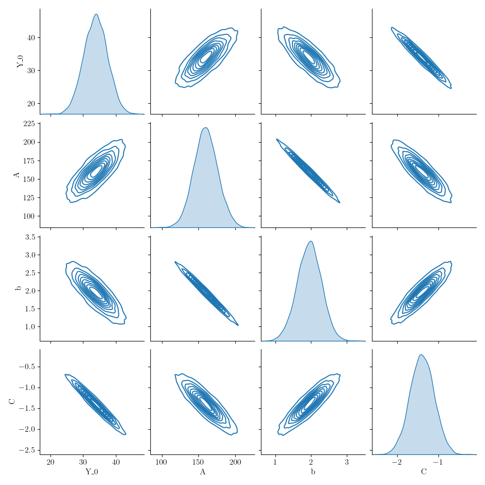
Next, we sample the multivariate normal provided by the study covariance and previous result mean and visualize the results using seaborn’s KDE pair plot
num_samples=5000
uncertain_param_sets = sample_multivariate_normal(num_samples,
                                                  laplace_results.mean.to_list(),
                                                  laplace_results.fitted_parameter_covariance,
                                                  12345,
                                                  params.get_item_names())
import seaborn as sns
import pandas as pd
sns.pairplot(data=pd.DataFrame(uncertain_param_sets), kind="kde" )
plt.show()

# sphinx_gallery_thumbnail_number = 3
/gpfs/knkarls/projects/matcal_devel/external_matcal/matcal/core/parameter_studies.py:918: RuntimeWarning: covariance is not symmetric positive-semidefinite.
  samples = rng.multivariate_normal(mean, sigma, nsamples).T
Total running time of the script: (5 minutes 25.156 seconds)