Uniaxial Tension Models

MatCal’s RoundUniaxialTensionModel and RectangularUniaxialTensionModel are meant to be used in calibrations requiring the simulation of a uniaxial tension test. These models have all the MatCal standard model features as described in MatCal SIERRA Solid Mechanics Standard Models. In this section, we will provide more information about how the geometries are generated, specifics on simulation boundary conditions, and what is output from these models.

Note

Some examples and V&V studies that include these models are:

1. 304L annealed bar viscoplastic calibrations

2. 6061T6 aluminum plate calibrations

3. MatCal Generated Models V&V Activities

Uniaxial tension geometry and mesh generation

Both of these models require very similar geometry parameters and are meshed in very similar ways. For their geometry to be accurately built, the models require the following keyword arguments be provided to their constructor.

1. total_length

2. gauge_length

3. extensometer_length

4. fillet_radius

5. taper - Specifies the taper from the target gauge width/radius at the center of the specimen gauge section to the ends of the gauge length where the gauge width/diameter increase by this value.

6. grip_contact_length - distance that the grips contact the specimen in the grip section.

7. necking_region (optional) - the fraction of the extensometer length where necking is expected to occur. This is used for output and mesh refinement for some of the mesh_methods.

8. element_size - target element edge length

9. mesh_method - user specified meshing method options

The necking_region geometry input is optional for these models. It specifies the fraction of the extensometer length where necking is expected to occur and is used for output and mesh refinement for some of the mesh_methods. If the user does not provide necking_region or provides a value of zero, MatCal automatically selects a default value. For the uniaxial tension models, the preferred default is 0.375. If 0.375 is outside the allowable range for the specified geometry and mesh size, MatCal instead selects the midpoint of the valid interval for necking_region. If the user provides a valid, nonzero necking_region, that value is used directly.

Keyword arguments specific to the RoundUniaxialTensionModel include those shown below.

1. gauge_radius

2. grip_radius

These parameters provide information related to geometry, discretization sizing and output and boundary condition mesh entities such as blocks and node sets. The geometric parameters for the RoundUniaxialTensionModel are shown in Fig. 3.

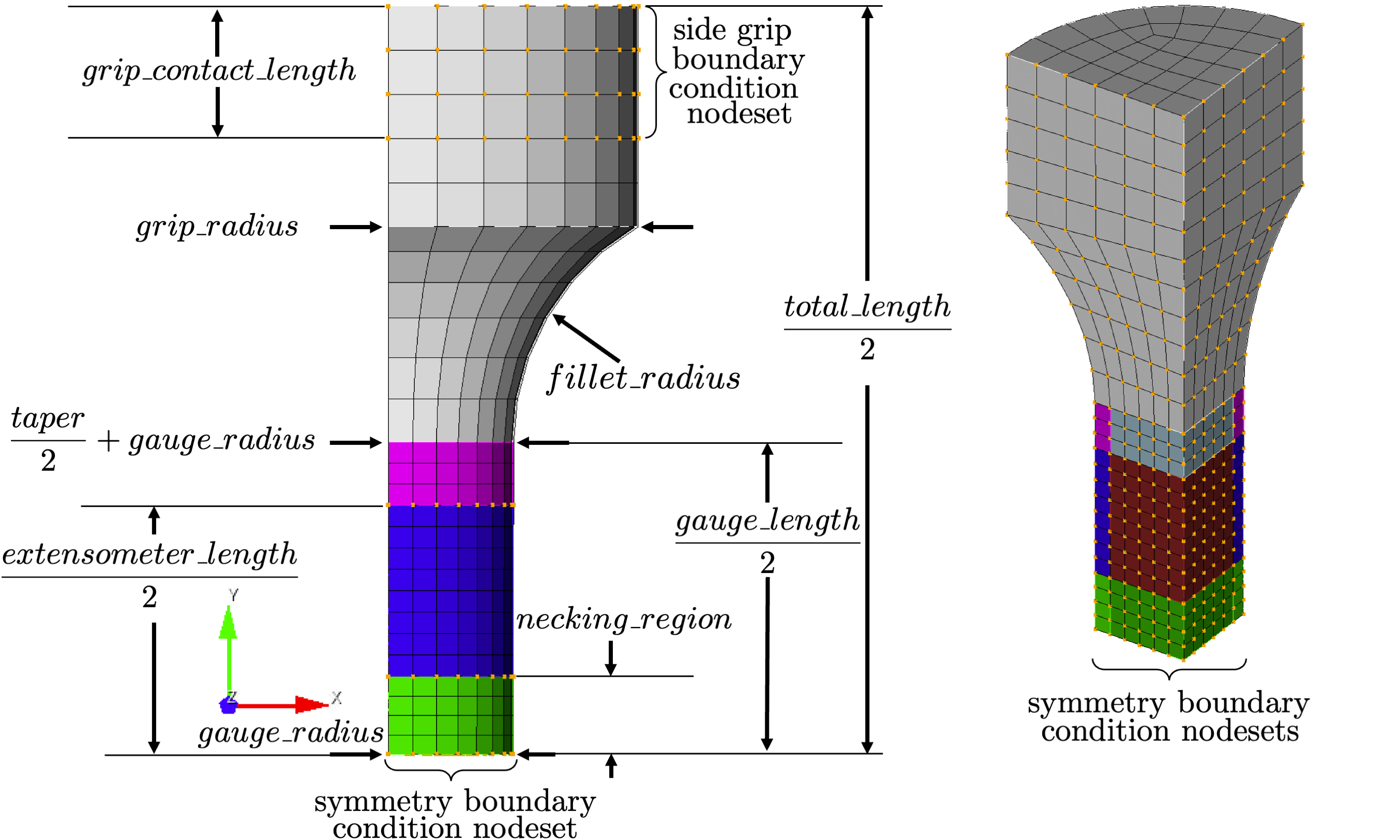
Fig. 3 The geometric dimensions and boundary conditions for the round cross-section model.

Similarly, arguments specific to the RectangularUniaxialTensionModel are as follows.

1. grip_width

2. gauge_width

3. thickness

The geometric parameters for the RectangularUniaxialTensionModel are shown in Fig. 4.

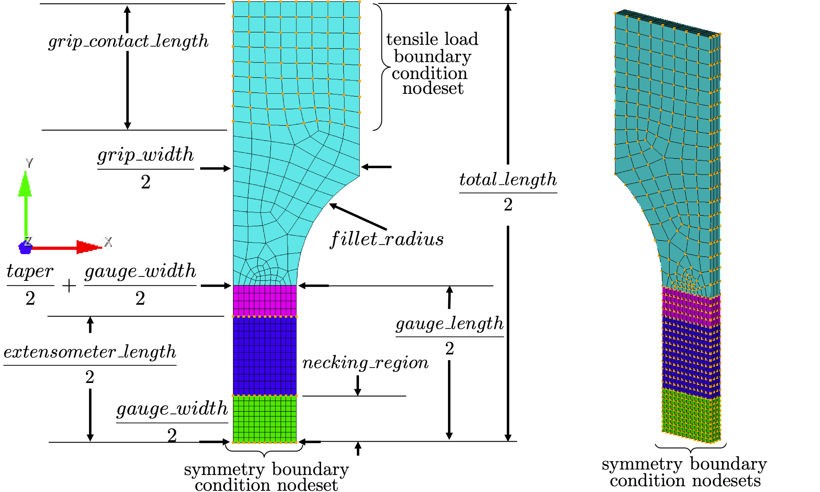
Fig. 4 The geometric dimensions and boundary conditions for the rectangular cross-section model.

The keyword element_size is used to specify the approximate element edge length that Cubit will target in the mesh. Depending on the meshing_method chosen, this could be the entire model or just a subregion of the model. The meshing_method parameter allows the user to change how the geometry is meshed. Differences in the 5 meshing_method available are shown in Fig. 5 and Fig. 6. In general, low meshing_method parameters are intended for coarser meshes and result in higher element counts. In contrast, high meshing_method parameters are intended for finer meshes, result in lower element counts and begin to use Cubit numsplits for meshing_method >= 4. Note that higher number mesh_methods can result in lower resolution of geometry away from the gauge section of the specimen if the target mesh size is too coarse.

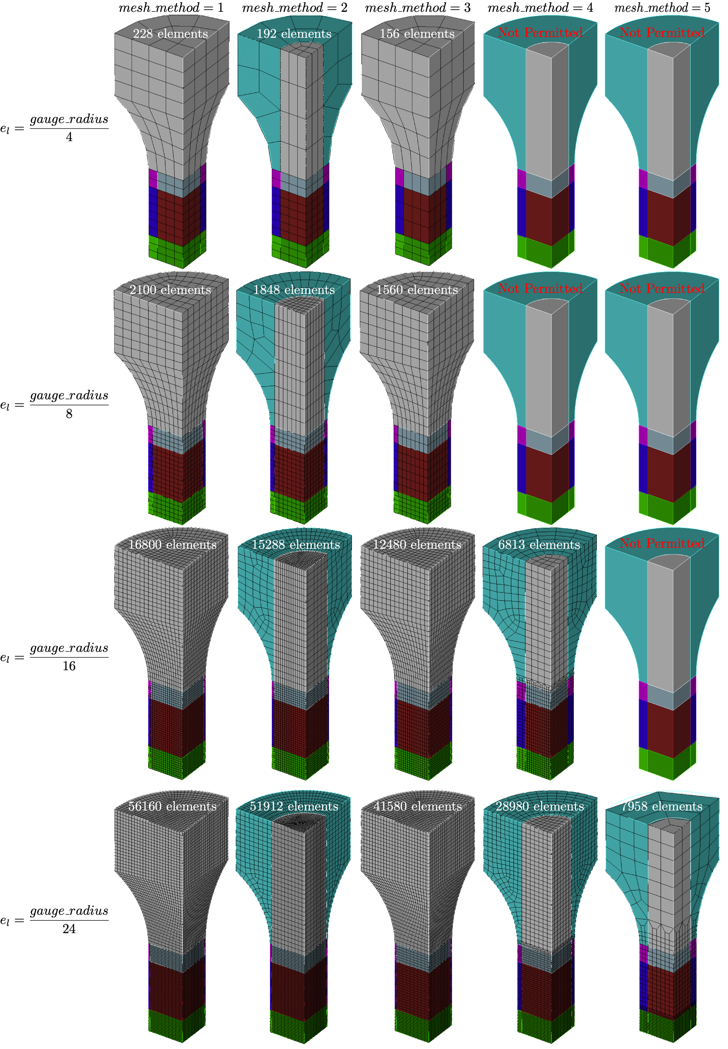
Fig. 5 The resulting meshes for different mesh_method options for the round cross-section model.

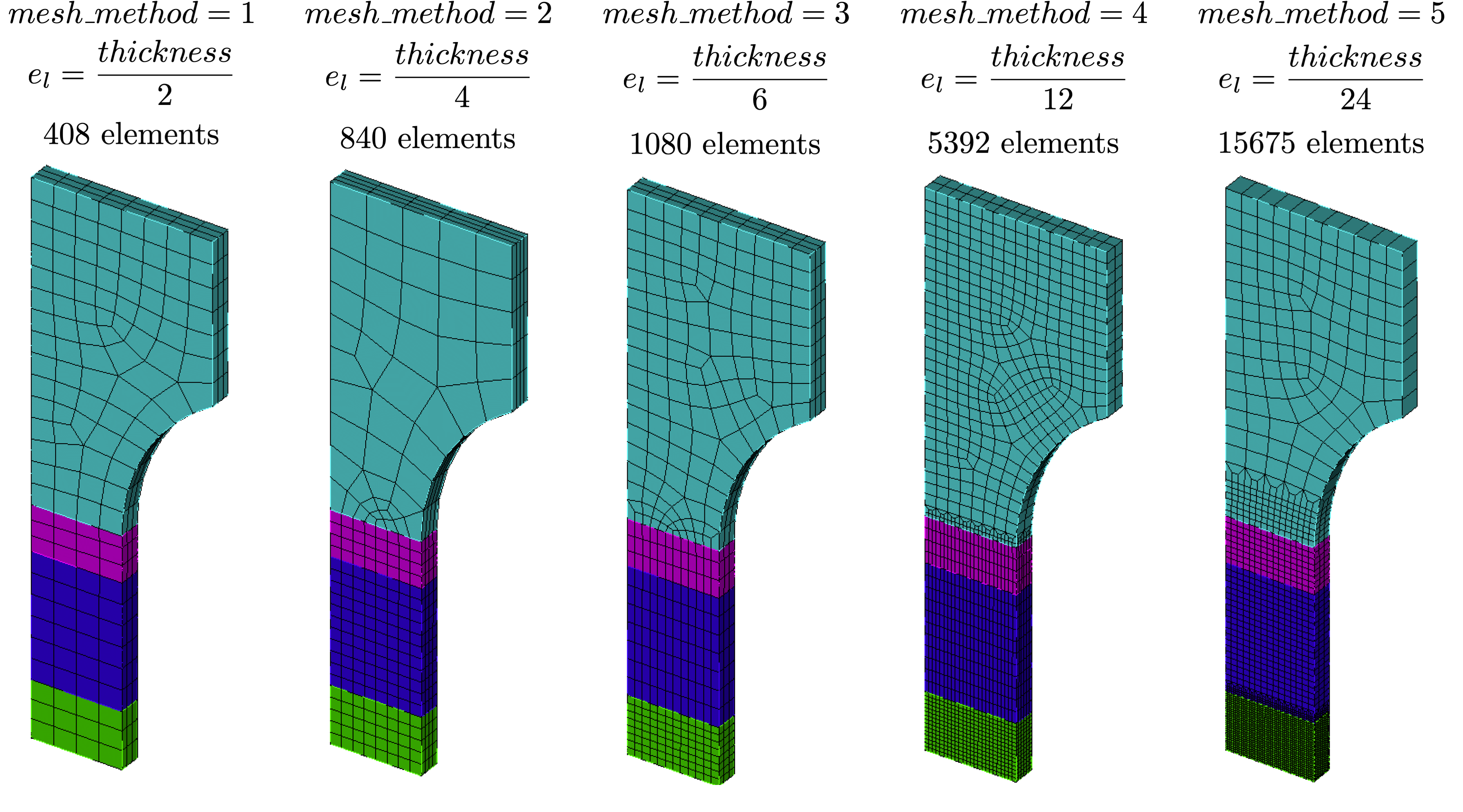
Fig. 6 The resulting meshes for different mesh_method options for the rectangular cross-section model.

Currently, the entire geometry is meshed in order to support thermomechanical coupling. Since conduction into the grips and load frame may be non-negligible, the entire specimen is important to model. We have found the extra computational cost associated with including the grips to be small.

Uniaxial tension boundary conditions

The tension models currently only support symmetry geometry, and, as a result, have boundary conditions that reflect that. The boundary conditions are shown graphically in Fig. 3 and Fig. 4. Since these models can easily be coupled with thermal modeling, the boundary condition descriptions have been separated into the following two subsections associated with the solid mechanics and thermal models.

Uniaxial tension solid mechanics boundary conditions

The tensile loading is caused by a displacement function applied to the outer surface of the grip section block in the axial direction away from the specimen center. This function acts on the surface of the specimen where the grips would contact it, and includes nodes from the top of the specimen down by the grip_contact_length dimension. For the round specimen, this includes all nodes on the outside radius of the grip section. For the rectangular specimen, this includes the nodes on the wide grip surface but not on the side grip surface that have a width equal to thickness. These node sets are shown for the two tension specimens in Fig. 3 and Fig. 4.

The applied function is determined using the add_boundary_condition_data(). This method must be supplied a Data or DataCollection class that contains either “engineering_strain” or “displacement” fields for the states of interest for the model. They can also optionally include a “time” field. The add_boundary_condition_data() method determines the boundary condition function to be applied to the tension specimens according to the following algorithm:

1. Determine the boundary condition by state since maximum deformation, material behavior and experiment setup can vary significantly over different states.

2. For each state, find the data set with the largest displacement/strain and use it for boundary condition generation.

3. If displacement data is provided, select it for the boundary condition generation and ignore engineering strain data. MatCal automatically scales the displacement by the gauge_length/extensometer_length This assumes that the strain is uniform throughout the gauge section for most of the load history and is intended to ensure that enough displacement is applied to the grips to achieve the desired displacement across the extensometer length.

4. If displacement data is not provided, use engineering strain for boundary condition generation and convert it to displacement using the geometry gauge_length. Once again this is to ensure enough displacement is applied to the specimen to achieve the correct deformation across the extensometer length.

5. If the data does not contain a “time” field and there is not a State parameter named “displacement_rate”, then apply a linear displacement function from zero to the maximum displacement found in the data over one second.

6. If the data does not contain a “time” field and there is a State parameter named “displacement_rate” or “engineering_strain_rate”, then apply a linear displacement function from zero to the maximum displacement found in the data. For “displacement_rate”, this is done over a time period beginning at zero seconds and ending at a time calculated by dividing the maximum displacement at the extensometer by the “displacement_rate” State parameter. For “engineering_strain_rate”, this is done over a time period calculated by dividing the maximum engineering strain by “engineering_strain_rate” and the specimen is displaced to a maximum displacement of the maximum engineering strain times gauge_length.

7. If the data does contain a “time” field, use the function directly as provided after scaling the “displacement” or “engineering_strain” fields such that they account for deformation in the gauge_length outside of the extensometer_length.

Note

This algorithm assumes that negligible deformation occurs in the regions outside of the specimen gauge length. If this is known or suspected to be an invalid assumption, an additional scale factor can be applied to increase the displacement applied to the grips. Use the set_boundary_condition_scale_factor() method to add a scale factor to scale the displacement function. It must be between 1 and 10 and it directly multiplies the displacement determined from the boundary condition generation algorithm.

The remaining solid mechanics boundary conditions only include the symmetry boundary conditions where displacements normal to the symmetry surfaces are set to zero.

Uniaxial tension thermal model boundary conditions

Since MatCal SIERRA/SM standard models only allow heat flux out of the specimen through the grips, only the grip boundary condition is described here. As discussed in the previous section, the boundary condition for the grip-to-specimen interface includes the nodes between the ends of the tension specimen model and grip_contact_length away from the ends of the specimen. As described in Staggered and iterative coupling, the temperature at the nodes is fixed to the value of the State parameter “temperature”. The entire body of the model is prescribed an initial temperate of State parameter “temperature” for all simulations regardless of coupling specification (uncoupled, staggered coupling, iterative coupling or adiabatic). For uncoupled simulations, this is only done if a temperature state variable is provided.

Uniaxial tension model specific output

By default, the tension models include the following global output fields:

1. time

2. displacement - measured across extensometer length in the loading direction

3. load - measured at the applied boundary condition node set in the loading direction.

4. engineering_strain - displacement divided by extensometer_length

5. engineering_stress - load divided by the gauge section center cross-sectional area.

If coupling is activated, the following global temperature output is provided:

1. low_temperature

2. med_temperature

3. high_temperature

and how they are calculated is dependent on the type of coupling. For adiabatic simulations, they are the minimum, average and maximum element temperatures in the gauge section of the model. For coupled simulations, the same quantities are provided by acting on the nodal temperatures instead of the element temperatures.