Note
Go to the end to download the full example code.
304L stainless steel mesh and time step convergence
Note
Useful Documentation links:
Mesh and time step convergence studies are an important part of the calibration process. Preliminary calibrations can usually be performed with a computationally inexpensive form of the model even if some error is introduced. However, at some point, the calibration should be finished with a model that is known to have a low discretization error. MatCal has tools to help perform these mesh and time step discretization studies.
This example is a continuation of the 304L stainless steel viscoplastic calibration example. Here we perform mesh and time step convergence on the tension model used for that study, and decide if a recalibration is necessary based on the discretization error present in the tension model used for the calibration. Since the discretization convergence studies only apply to the tension model, we leave out the yield versus rate python model and its associated data and objective.
To begin, the data import, model preparation and objective specification for the tension model from the original calibration are repeated.
import matplotlib.pyplot as plt
import numpy as np
from matcal import *

plt.rc('text', usetex=True)
plt.rc('font', family='serif')
plt.rc('font', size=12)
figsize = (5,4)

tension_data = BatchDataImporter("ductile_failure_ASTME8_304L_data/*.dat",
                                    file_type="csv")
tension_data.set_fixed_state_parameters(displacement_rate=2e-4, temperature=530)
tension_data = tension_data.batch
tension_data = scale_data_collection(tension_data, "engineering_stress", 1000)
tension_data.remove_field("time")

material_name = "304L_viscoplastic"
material_filename = "304L_viscoplastic_voce_hardening.inc"
sierra_material = Material(material_name, material_filename,
                            "j2_plasticity")

geo_params = {"extensometer_length": 0.75,
               "gauge_length": 1.25,
               "gauge_radius": 0.125,
               "grip_radius": 0.25,
               "total_length": 4,
               "fillet_radius": 0.188,
               "taper": 0.0015,
               "necking_region":0.375,
               "element_size": 0.02,
               "mesh_method":3,
               "grip_contact_length":1}

astme8_model = RoundUniaxialTensionModel(sierra_material, **geo_params)
astme8_model.add_boundary_condition_data(tension_data)
astme8_model.set_allowable_load_drop_factor(0.25)
astme8_model.set_name("ASTME8_tension_model")
astme8_model.add_constants(ref_strain_rate=1e-5)
astme8_model.add_constants(element_size=0.01, mesh_method=4)

from site_matcal.sandia.computing_platforms import is_sandia_cluster, get_sandia_computing_platform
from site_matcal.sandia.tests.utilities import MATCAL_WCID

cores_per_node = 24
if is_sandia_cluster():
    platform = get_sandia_computing_platform()
    cores_per_node = platform.processors_per_node
    astme8_model.run_in_queue(MATCAL_WCID, 2)
    astme8_model.continue_when_simulation_fails()
astme8_model.set_number_of_cores(cores_per_node)

objective = CurveBasedInterpolatedObjective("engineering_strain", "engineering_stress")
objective.set_name("stress_objective")

def remove_uncalibrated_data_from_residual(engineering_strains, engineering_stresses,
                                           residuals):
    import numpy as np
    weights = np.ones(len(residuals))
    weights[engineering_stresses < 38e3] = 0
    weights[engineering_strains > 0.75] = 0
    return weights*residuals

residual_weights = UserFunctionWeighting("engineering_strain", "engineering_stress",
                                         remove_uncalibrated_data_from_residual)
objective.set_field_weights(residual_weights)
Now to setup the mesh convergence study, we will use Python’s copy module to copy the astme8_model and modify the element sizes for the new models. If needed, we can also change the number of cores to be used for each model.
from copy import deepcopy

astme8_model_coarse = deepcopy(astme8_model)
astme8_model_coarse.add_constants(element_size=0.02, mesh_method=3)
if is_sandia_cluster():
    astme8_model_coarse.run_in_queue(MATCAL_WCID, 0.5)
astme8_model_coarse.set_name("ASTME8_tension_model_coarse")


astme8_model_fine = deepcopy(astme8_model)
astme8_model_fine.add_constants(element_size=0.005, mesh_method=4)
if is_sandia_cluster():
    astme8_model_fine.run_in_queue(MATCAL_WCID, 4)
    astme8_model_fine.set_number_of_cores(cores_per_node*2)
astme8_model_fine.set_name("ASTME8_tension_model_fine")

astme8_model_finest = deepcopy(astme8_model)
astme8_model_finest.add_constants(element_size=0.0025, mesh_method=4)
if is_sandia_cluster():
    astme8_model_finest.run_in_queue(MATCAL_WCID, 4)
    astme8_model_finest.set_number_of_cores(cores_per_node*4)
astme8_model_finest.set_name("ASTME8_tension_model_finest")
We will then perform a ParameterStudy
where the only parameters
to be evaluated are the calibrated parameters from the initial study.
calibrated_params = matcal_load("voce_calibration_results.serialized")
Y_0_val = calibrated_params["Y_0"]
Y_0 = Parameter("Y_0", Y_0_val*0.9, Y_0_val*1.1, Y_0_val)

A_val = calibrated_params["A"]
A = Parameter("A", A_val*0.9, A_val*1.1, A_val)

b_val = calibrated_params["b"]
b = Parameter("b", 1.5, 2.5, b_val)

C_val = calibrated_params["C"]
C = Parameter("C", C_val*1.1, C_val*0.9, C_val)
The X parameter is not needed, so it is removed from the calibration parameter dictionary.
calibrated_params.pop("X")

param_study = ParameterStudy(Y_0, A, b, C)
param_study.set_results_storage_options(weighted_conditioned=True)
param_study.add_parameter_evaluation(**calibrated_params)
This mesh discretization study will need to evaluate all models we created, so each is added to the study as their own evaluation set.
param_study.add_evaluation_set(astme8_model_coarse, objective,
                               tension_data)
param_study.add_evaluation_set(astme8_model, objective,
                               tension_data)
param_study.add_evaluation_set(astme8_model_fine, objective,
                               tension_data)
param_study.add_evaluation_set(astme8_model_finest, objective,
                               tension_data)
Lastly, the study core limit is set appropriately. The core limit is set to 112 cores which is what our hardware can support.
param_study.set_core_limit(112)
param_study.set_working_directory("mesh_study", remove_existing=True)
We can now run the study. After it finishes, we can make our convergence plot.
mesh_results = param_study.launch()
For our purposes, we want to ensure that the objective value is converged or has an acceptable error. As a result, we manipulate the results output from this study to access the objective values for each mesh size, the engineering stress-strain curves from the data and the residuals from the evaluations. We want to plot the residuals for each model as a function of the engineering strain for two of the samples, R2S1 and R4S2. Since the residuals for each model are calculated at the experimental data independent variables, their engineering strain values will be the same for all data sets.
state = tension_data.state_names[0]
resid_exp_qois = mesh_results.get_experiment_qois(astme8_model, objective, state)
resid_strain_R2S1 = resid_exp_qois[2]["engineering_strain"]
resid_strain_R4S2 = resid_exp_qois[7]["engineering_strain"]
For the residual values and simulation data we will have to extract the data from the results object for each model. We write a function to perform this data extraction on a provided model and retrun the results.
def get_data_and_residuals_results_by_model(model, results):
    obj = results.best_evaluation_set_objective(model, objective)
    curves = results.best_simulation_data(model, state)

    resids_R2S1 = results.best_residuals(model, objective, state, 2)
    resids_R4S2 = results.best_residuals(model, objective, state, 7)
    weight_cond_resids_R2S1 = results.best_weighted_conditioned_residuals(model, objective,
                                                                          state, 2)

    weight_cond_resids_R4S2 = results.best_weighted_conditioned_residuals(model, objective,
                                                                          state, 7)

    return (obj, curves, resids_R2S1, resids_R4S2,
            weight_cond_resids_R2S1, weight_cond_resids_R4S2)
Next, we apply the function to each model and organize the data for plotting.
coarse_results = get_data_and_residuals_results_by_model(astme8_model_coarse,
                                                         mesh_results)
coarse_objective_results = coarse_results[0]
coarse_curves = coarse_results[1]
coarse_resids_R2S1 = coarse_results[2]
coarse_resids_R4S2 = coarse_results[3]
coarse_weight_cond_resids_R2S1 = coarse_results[4]
coarse_weight_cond_resids_R4S2 = coarse_results[5]

orig_results = get_data_and_residuals_results_by_model(astme8_model,
                                                         mesh_results)
orig_objective_results = orig_results[0]
orig_curves = orig_results[1]
orig_resids_R2S1 = orig_results[2]
orig_resids_R4S2 = orig_results[3]
orig_weight_cond_resids_R2S1 = orig_results[4]
orig_weight_cond_resids_R4S2 = orig_results[5]

fine_results = get_data_and_residuals_results_by_model(astme8_model_fine,
                                                         mesh_results)
fine_objective_results = fine_results[0]
fine_curves = fine_results[1]
fine_resids_R2S1 = fine_results[2]
fine_resids_R4S2 = fine_results[3]
fine_weight_cond_resids_R2S1 = fine_results[4]
fine_weight_cond_resids_R4S2 = fine_results[5]

finest_results = get_data_and_residuals_results_by_model(astme8_model_finest,
                                                         mesh_results)
finest_objective_results = finest_results[0]
finest_curves = finest_results[1]
finest_resids_R2S1 = finest_results[2]
finest_resids_R4S2 = finest_results[3]
finest_weight_cond_resids_R2S1 = finest_results[4]
finest_weight_cond_resids_R4S2 = finest_results[5]
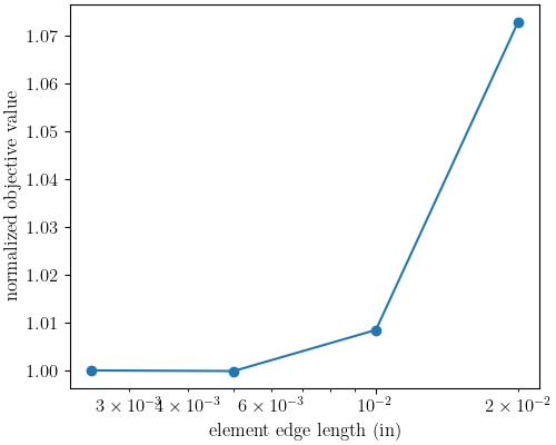
We then use Matplotlib [9] to plot the objective values versus the element size.
time_steps = np.array([0.02, 0.01, 0.005, 0.0025])
objectives = np.array([coarse_objective_results, orig_objective_results,
                       fine_objective_results, finest_objective_results])
plt.figure(figsize=figsize,constrained_layout=True)
plt.semilogx(time_steps, objectives/finest_objective_results, 'o-')
plt.xlabel("element edge length (in)")
plt.ylabel("normalized objective value")
/gpfs/knkarls/projects/matcal_devel/external_matcal/documentation/advanced_examples/304L_viscoplastic_calibration/plot_304L_d_tension_convergence_study_cluster.py:262: RuntimeWarning: invalid value encountered in divide
  plt.semilogx(time_steps, objectives/finest_objective_results, 'o-')

Text(18.92641051136365, 0.5, 'normalized objective value')
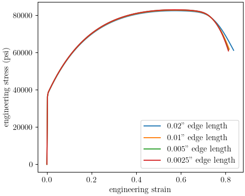
We also plot the raw simulation stress/strain curves. Note that this is different than the simulation QoIs used for the objective since the QoIs are the simulation curves interpolated to the experiment strain points.
plt.figure(figsize=figsize,constrained_layout=True)
plt.plot(coarse_curves["engineering_strain"],
         coarse_curves["engineering_stress"], label="0.02\" edge length")
plt.plot(orig_curves["engineering_strain"],
         orig_curves["engineering_stress"], label="0.01\" edge length")
plt.plot(fine_curves["engineering_strain"],
         fine_curves["engineering_stress"], label="0.005\" edge length")
plt.plot(finest_curves["engineering_strain"],
         finest_curves["engineering_stress"], label="0.0025\" edge length")
plt.xlabel("engineering strain")
plt.ylabel("engineering stress (psi)")
plt.legend()
<matplotlib.legend.Legend object at 0x155511d140e0>
These plots show the objective is converging with reduced element size and the objective values change ~1% or less with element size less than or equal to 0.005”. As a result, we will consider the model with the 0.005” elements to be accurate enough for our calibration purposes.
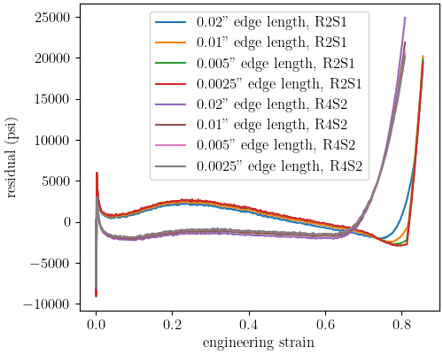
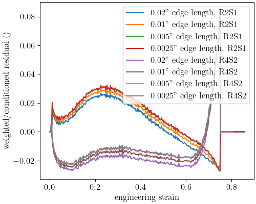
Finally, we plot the residuals for two of the experimental data sets, R2S1 and R4S2, by mesh size. to see if any portion of the stress-strain curve is more mesh sensitive. We also plot the weighted and conditioned residuals to observe the effect of the weighting applied.
plt.figure(figsize=figsize,constrained_layout=True)
plt.plot(resid_strain_R2S1, coarse_resids_R2S1["engineering_stress"],
          label="0.02\" edge length, R2S1")
plt.plot(resid_strain_R2S1, orig_resids_R2S1["engineering_stress"],
         label="0.01\" edge length, R2S1")
plt.plot(resid_strain_R2S1, fine_resids_R2S1["engineering_stress"],
         label="0.005\" edge length, R2S1")
plt.plot(resid_strain_R2S1, finest_resids_R2S1["engineering_stress"],
         label="0.0025\" edge length, R2S1")
plt.plot(resid_strain_R4S2, coarse_resids_R4S2["engineering_stress"],
         label="0.02\" edge length, R4S2")
plt.plot(resid_strain_R4S2, orig_resids_R4S2["engineering_stress"],
         label="0.01\" edge length, R4S2")
plt.plot(resid_strain_R4S2, fine_resids_R4S2["engineering_stress"],
         label="0.005\" edge length, R4S2")
plt.plot(resid_strain_R4S2, finest_resids_R4S2["engineering_stress"],
         label="0.0025\" edge length, R4S2")
plt.xlabel("engineering strain")
plt.ylabel("residual (psi)")
plt.legend()
<matplotlib.legend.Legend object at 0x155511bedd90>
In this first plot, it is clear that the residuals
are highest near the regions that were removed
using the UserFunctionWeighting
object. However, the residual behavior in the two regions differ
because little variability is displayed in the elastic region for the two observed
data sets and different mesh sizes
while at the unloading portion of the curve the residuals
are much more sensitive to data set and mesh size. In fact,
the raw residuals are clearly not converging in this region.
plt.figure(figsize=figsize,constrained_layout=True)
plt.plot(resid_strain_R2S1, coarse_weight_cond_resids_R2S1["engineering_stress"],
         label="0.02\" edge length, R2S1")
plt.plot(resid_strain_R2S1, orig_weight_cond_resids_R2S1["engineering_stress"],
         label="0.01\" edge length, R2S1")
plt.plot(resid_strain_R2S1, fine_weight_cond_resids_R2S1["engineering_stress"],
         label="0.005\" edge length, R2S1")
plt.plot(resid_strain_R2S1, finest_weight_cond_resids_R2S1["engineering_stress"],
         label="0.0025\" edge length, R2S1")
plt.plot(resid_strain_R4S2, coarse_weight_cond_resids_R4S2["engineering_stress"],
         label="0.02\" edge length, R4S2")
plt.plot(resid_strain_R4S2, orig_weight_cond_resids_R4S2["engineering_stress"],
         label="0.01\" edge length, R4S2")
plt.plot(resid_strain_R4S2, fine_weight_cond_resids_R4S2["engineering_stress"],
         label="0.005\" edge length, R4S2")
plt.plot(resid_strain_R4S2, finest_weight_cond_resids_R4S2["engineering_stress"],
         label="0.0025\" edge length, R4S2")
plt.xlabel("engineering strain")
plt.ylabel("weighted/conditioned residual ()")
plt.legend()
<matplotlib.legend.Legend object at 0x1555119740e0>
In the second plot, the weighting has removed parts of the problematic portions of the stress-strain curve as discussed in the original calibration example. A significant portion of the elastic region and unloading region of the data no longer contributes to the residual. Although the elastic region of the curve likely had no effect on this convergence study, not removing the tail end of the unloading region likely would have prevented convergence for this problem and meshes studied.
With the mesh size selected, a similar study can also be performed for time step convergence. We start by first updating the model constants from each model to the mesh size selected above. We can then change the number of time steps the models will target.
if is_sandia_cluster():
    astme8_model_coarse.run_in_queue(MATCAL_WCID, 2)
    astme8_model_coarse.set_number_of_cores(cores_per_node*2)
astme8_model_coarse.add_constants(element_size=0.005, mesh_method=4)
astme8_model_coarse.set_number_of_time_steps(150)

astme8_model.set_number_of_time_steps(300)
astme8_model.add_constants(element_size=0.005, mesh_method=4)
if is_sandia_cluster():
    astme8_model.run_in_queue(MATCAL_WCID, 4)
    astme8_model.set_number_of_cores(cores_per_node*2)

astme8_model_fine.set_number_of_time_steps(600)
if is_sandia_cluster():
    astme8_model_fine.run_in_queue(MATCAL_WCID, 4)
    astme8_model_fine.set_number_of_cores(cores_per_node*3)
astme8_model_fine.add_constants(element_size=0.005, mesh_method=4)

astme8_model_finest = deepcopy(astme8_model_fine)
astme8_model_finest.set_number_of_time_steps(1200)
if is_sandia_cluster():
    astme8_model_finest.run_in_queue(MATCAL_WCID, 4)
    astme8_model_finest.set_number_of_cores(cores_per_node*4)
astme8_model_finest.add_constants(element_size=0.005, mesh_method=4)
astme8_model_finest.set_name("ASTME8_tension_model_finest")
Next, we re-create a new study to be launched with the updated models.
param_study = ParameterStudy(Y_0, A, b, C)
param_study.set_results_storage_options(weighted_conditioned=True)
param_study.add_parameter_evaluation(**calibrated_params)
param_study.add_evaluation_set(astme8_model_coarse,
                               objective, tension_data)
param_study.add_evaluation_set(astme8_model,
                               objective, tension_data)
param_study.add_evaluation_set(astme8_model_fine,
                               objective, tension_data)
param_study.add_evaluation_set(astme8_model_finest,
                               objective, tension_data)
param_study.set_core_limit(112)
param_study.set_working_directory("time_step_study", remove_existing=True)

time_step_results = param_study.launch()
Once again, we can make our
convergence plot using Matplotlib after
extracting the desired data from the study results.
The number of time steps specified using the model method
set_number_of_time_steps()
is only a target number of time steps. The model may change this with
adaptive time stepping which is used to increase model reliability.
As a result, we
obtain two values from each completed model for the convergence plot: the number of actual
time steps that the simulation took and the objective for that result. Once again, we
also plot the simulation data curves for each case.
coarse_results = get_data_and_residuals_results_by_model(astme8_model_coarse,
time_step_results)
coarse_objective_results = coarse_results[0]
coarse_curves = coarse_results[1]
coarse_num_time_steps = len(coarse_curves)
orig_results = get_data_and_residuals_results_by_model(astme8_model,
time_step_results)
orig_objective_results = orig_results[0]
orig_curves = orig_results[1]
mid_num_time_steps = len(orig_curves)
fine_results = get_data_and_residuals_results_by_model(astme8_model_fine,
time_step_results)
fine_objective_results = fine_results[0]
fine_curves = fine_results[1]
fine_num_time_steps = len(fine_curves)
finest_results = get_data_and_residuals_results_by_model(astme8_model_finest,
time_step_results)
finest_objective_results = finest_results[0]
finest_curves = finest_results[1]
finer_num_time_steps = len(finest_curves)
plt.figure(figsize=figsize,constrained_layout=True)
time_steps = np.array([coarse_num_time_steps, mid_num_time_steps,
fine_num_time_steps, finer_num_time_steps])
objectives = np.array([coarse_objective_results, orig_objective_results,
fine_objective_results, finest_objective_results])
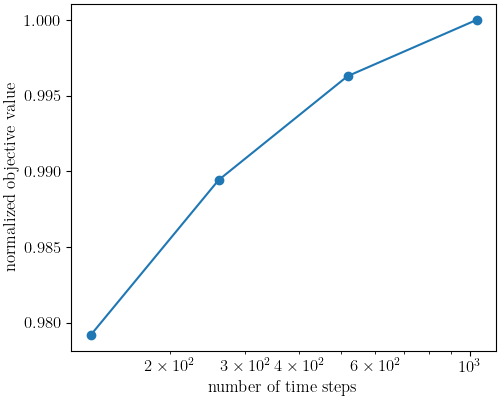
plt.semilogx(time_steps, objectives/finest_objective_results, 'o-')
plt.xlabel("number of time steps")
plt.ylabel("normalized objective value")
plt.figure(figsize=figsize, constrained_layout=True)
plt.plot(coarse_curves["engineering_strain"], coarse_curves["engineering_stress"],
label=f"{coarse_num_time_steps} time steps")
plt.plot(orig_curves["engineering_strain"], orig_curves["engineering_stress"],
label=f"{mid_num_time_steps} time steps")
plt.plot(fine_curves["engineering_strain"], fine_curves["engineering_stress"],
label=f"{fine_num_time_steps} time steps")
plt.plot(finest_curves["engineering_strain"], finest_curves["engineering_stress"],
label=f"{finer_num_time_steps} time steps")
plt.xlabel("engineering strain")
plt.ylabel("engineering stress (psi)")
plt.legend()
plt.show()

/gpfs/knkarls/projects/matcal_devel/external_matcal/documentation/advanced_examples/304L_viscoplastic_calibration/plot_304L_d_tension_convergence_study_cluster.py:452: RuntimeWarning: invalid value encountered in divide
  plt.semilogx(time_steps, objectives/finest_objective_results, 'o-')
These plots show the objective is converging with increased time steps and the objective value change becomes ~1% or less with 300 or more time steps. As a result, we will consider the model with 300 or more time steps to be accurate enough for our calibration purposes. This happens to be the default value for the MatCal generated models’ target number of time steps. Note that the converged number of time steps will be boundary value problem dependent and time step convergence should always be performed as part of the calibration process. Based on these findings, the calibration can be finalized with a recalibration using a model with element sizes of 0.005” and more than 300 time steps.
Total running time of the script: (96 minutes 26.856 seconds)