6061T6 aluminum calibration uncertainty quantification

In this example, we will use MatCal’s LaplaceStudy to estimate the parameter uncertainty for the calibration.

This uncertainty quantification study differs from the one in 304L stainless steel viscoplastic calibration uncertainty quantification because many of the parameters are directly correlated to other parameters in the model. Specifically, the temperature and anisotropy parameters, are multipliers of the yield stress and Voce hardening parameters. As a result, we will assume all parameter uncertainty can be attributed to the yield stress and Voce hardening parameters alone. This will significantly reduce the cost of the finite difference calculations needed for the LaplaceStudy and ensure robustness of the method.

We want the uncertainty in these three parameters to account for all uncertainty in the room temperature experiments, so we include these models in the uncertainty study.

Warning

The LaplaceStudy is still in development and may not accurately attribute uncertainty to to the parameters. Always verify results before use.

Note

Useful Documentation links:

1. Uniaxial Tension Models

2. Top Hat Shear Model

3. LaplaceStudy

To begin, we import the tools we need for this study.

from matcal import *
from site_matcal.sandia.computing_platforms import is_sandia_cluster, get_sandia_computing_platform
from site_matcal.sandia.tests.utilities import MATCAL_WCID

import numpy as np
import matplotlib.pyplot as plt

plt.rc('text', usetex=True)
plt.rc('font', family='serif')
plt.rc('font', size=12)
figsize = (4,3)

Next, we import the data and remove any uncalibrated data from the DataCollection objects. We do this in place of weighting, because zeros in the residuals can cause scaling and conditioning issues in the linear algebra required for the study.

tension_data_collection = BatchDataImporter("aluminum_6061_data/"
                                              "uniaxial_tension/processed_data/"
                                              "cleaned_[CANM]*.csv",).batch

For the room temperature tension data, we remove data in the elastic region and in regions of unloading to match what was included in the objective for the calibration.

down_selected_tension_data = DataCollection("down selected data")
for state in tension_data_collection.keys():
    for index, data in enumerate(tension_data_collection[state]):
        stresses = data["engineering_stress"]
        strains = data["engineering_strain"]
        peak_index = np.argmax(stresses)
        peak_strain = strains[peak_index]
        peak_stress = stresses[peak_index]
        data_to_keep = (((strains>peak_strain) & (stresses > 0.89*peak_stress)) |
                        (strains>0.005) & (strains < peak_strain))
        down_selected_tension_data.add(data[data_to_keep])

down_selected_tension_data = scale_data_collection(down_selected_tension_data,
                                                   "engineering_stress", 1000)
down_selected_tension_data.remove_field("time")

With the down-selected tension data created, we create the RoundUniaxialTensionModel as we did in 6061T6 aluminum calibration with anisotropic yield, and add the DataCollection that we created as the model boundary condition data.

material_filename = "hill_plasticity_temperature_dependent.inc"
material_model = "hill_plasticity"
material_name = "ductile_failure_6061T6"
sierra_material = Material(material_name, material_filename, material_model)

gauge_radius = 0.125
element_size = gauge_radius/8
geo_params = {"extensometer_length": 1.0,
              "gauge_length": 1.25,
              "gauge_radius": gauge_radius,
              "grip_radius": 0.25,
              "total_length": 4,
              "fillet_radius": 0.188,
              "taper": 0.0015,
              "necking_region":0.375,
              "element_size": element_size,
              "mesh_method":3,
              "grip_contact_length":1}

tension_model = RoundUniaxialTensionModel(sierra_material, **geo_params)
tension_model.set_name("tension_model")
tension_model.add_boundary_condition_data(down_selected_tension_data)
tension_model.set_allowable_load_drop_factor(0.70)
tension_model.set_boundary_condition_scale_factor(1.5)

if is_sandia_cluster():
  tension_model.run_in_queue(MATCAL_WCID, 1)
  tension_model.continue_when_simulation_fails()
  platform = get_sandia_computing_platform()
  num_cores = platform.get_processors_per_node()
else:
  num_cores = 8
tension_model.set_number_of_cores(num_cores)

Similarly, we import the top hat data and down select the data of interest for the residuals.

top_hat_data_collection = BatchDataImporter("aluminum_6061_data/"
                                              "top_hat_shear/processed_data/cleaned_*.csv").batch
for state, state_data_list in top_hat_data_collection.items():
    for index, data in enumerate(state_data_list):
        max_load_arg = np.argmax(data["load"])
        # This slicing procedure removes the data after peak load
        # and before displacements of 0.005".
        data = data[data["time"] < data["time"][max_load_arg]]
        data = data[data["displacement"] > 0.005]
        # This one removes the data after a displacement of 0.02"
        # and reassigns the modified data to the
        # DataCollection
        top_hat_data_collection[state][index] = data[data["displacement"] < 0.02]
top_hat_data_collection.remove_field("time")

With the data prepared, we can build the model as we did in the previous example 6061T6 aluminum calibration with anisotropic yield.

top_hat_geo_params = {"total_height":1.25,
        "base_height":0.75,
        "trapezoid_angle": 10.0,
        "top_width": 0.417*2,
        "base_width": 1.625,
        "base_bottom_height": (0.75-0.425),
        "thickness":0.375,
        "external_radius": 0.05,
        "internal_radius": 0.05,
        "hole_height": 0.3,
        "lower_radius_center_width":0.390*2,
        "localization_region_scale":0.0,
        "element_size":0.005,
        "numsplits":1}

top_hat_model = TopHatShearModel(sierra_material, **top_hat_geo_params)
top_hat_model.set_name('top_hat_shear')

Next, we set its allowable load drop factor and provide boundary condition data.

top_hat_model.set_allowable_load_drop_factor(0.05)
top_hat_model.add_boundary_condition_data(top_hat_data_collection)

Lastly, we setup the platform information for running the model.

top_hat_model.set_number_of_cores(num_cores*2)
if is_sandia_cluster():
  top_hat_model.run_in_queue(MATCAL_WCID, 1)
  top_hat_model.continue_when_simulation_fails()

We now create the objectives for the calibration. Both models are compared to the data using a CurveBasedInterpolatedObjective. The tension specimen is calibrated to the engineering stress/strain data and the top hat specimen is calibrated to the load-displacement data.

tension_objective = CurveBasedInterpolatedObjective("engineering_strain", "engineering_stress")
tension_objective.set_name("engineering_stress_strain_obj")
top_hat_objective = CurveBasedInterpolatedObjective("displacement", "load")
top_hat_objective.set_name("load_displacement_obj")

We now create our parameters for the study. The study parameters are the yield_stress, hardening and b parameters from 6061T6 aluminum calibration with anisotropic yield with their current value set to their calibration values.

RT_calibrated_params = matcal_load("anisotropy_parameters.serialized")
yield_stress = Parameter("yield_stress", 15, 50,
        RT_calibrated_params.pop("yield_stress"))
hardening = Parameter("hardening", 0, 60,
        RT_calibrated_params.pop("hardening"))
b = Parameter("b", 10, 40,
        RT_calibrated_params.pop("b"))

To simplify setting up the laplace study, we put all the parameters in a ParameterCollection.

pc = ParameterCollection("uncertain_params", yield_stress, hardening, b)

We also need the anisotropy so we store those parameters with the current value equal to the calibrated parameter values from the calibration step.

R22 = Parameter("R22", 0.8, 1.15,
        RT_calibrated_params["R22"])
R33 = Parameter("R33", 0.8, 1.15,
        RT_calibrated_params["R33"])
R12 = Parameter("R12", 0.8, 1.15,
        RT_calibrated_params["R12"])
R23 = Parameter("R23", 0.8, 1.15,
        RT_calibrated_params["R23"])
R31 = Parameter("R31", 0.8, 1.15,
        RT_calibrated_params["R31"])

The anisotropy parameters and temperature dependence parameters from 6061T6 aluminum temperature dependent calibration will be added as model constants because they are being treated as deterministic and are still required for the models. They are added for the two models for this study.

high_temp_calibrated_params = matcal_load("temperature_dependent_parameters.serialized")
tension_model.add_constants(**high_temp_calibrated_params,
                            **RT_calibrated_params)
top_hat_model.add_constants(**high_temp_calibrated_params,
                            **RT_calibrated_params)

Now we can create our laplace study and add our two evaluation sets.

laplace_study = LaplaceStudy(pc)
laplace_study.set_parameter_center(**pc.get_current_value_dict())
laplace_study.set_working_directory("laplace_study", remove_existing=True)
laplace_study.set_core_limit(250)
laplace_study.add_evaluation_set(tension_model, tension_objective, down_selected_tension_data)
laplace_study.add_evaluation_set(top_hat_model, top_hat_objective, top_hat_data_collection)

Laplace study specific options include set_step_size() to set the finite difference step size and set_noise_estimate() for setting the estimated amount of noise in the data. We set the finite difference step size to one order of magnitude less than the default. Results are likely sensitive to this value for practical problems, and re-running the study with different values may be required.

laplace_study.set_step_size(1e-4)

For this study type, providing an inaccurate noise estimate can result in unreasonable solutions.

Warning

Appropriately handling the noise estimate is an active area of research. If attempted, some iteration may be required to find an valid estimate for noise. This can be done by running the study once to evaluate the model response and then re-running the study as a restart after changing the noise estimate or by calling update_laplace_estimate().

laplace_study.set_noise_estimate(1e-2)
results = laplace_study.launch()

After the study completes, there are two results of concern:

1. The estimated parameter covariance - calculated directly from the residual magnitude and the gradients of the residuals w.r.t. the parameters.

2. The fitted parameter covariance - an optimized covariance that ensures the the covariance of the parameters is representative of the uncertainty due to model form error. This corrects the estimated parameter covariance using the objective described in Laplace Approximation: Error Attributed to Model Error

We print both of these values below and save the results to be used in the next step of this example.

print("Initial covariance estimate:\n", results.estimated_parameter_covariance)
print("Calibrated covariance estimate:\n", results.fitted_parameter_covariance)
matcal_save("laplace_study_results.joblib", results)

Initial covariance estimate:
 [[ 113.66447863  -20.90050619 -422.18930642]
 [ -20.90050619    5.62379061   70.41401601]
 [-422.18930642   70.41401601 1607.23724872]]
Calibrated covariance estimate:
 [[ 125.77931866  -22.62114298 -485.48255954]
 [ -22.62114298    5.84238658   77.55667787]
 [-485.48255954   77.55667787 1915.39817462]]

As noted above, the results can be sensitive to the estimated noise. To illustrate this point, we re-run the study results processing with updated noise estimates and print the results. Before updating the results, we save the previous results as copy of themselves because the update just updates the values on the results object.

import copy
results = copy.deepcopy(results)

results_high_noise = laplace_study.update_laplace_estimate(1e-1)
results_high_noise = copy.deepcopy(results_high_noise)

print("Initial covariance estimate noise set to 1e-2:\n", results.estimated_parameter_covariance)
print("Calibrated covariance estimate noise set to 1e-2:\n",
      results.fitted_parameter_covariance)

print("Initial covariance estimate noise set to 1e-1:\n", results_high_noise.estimated_parameter_covariance)
print("Calibrated covariance estimate noise set to 1e-1:\n",
      results_high_noise.fitted_parameter_covariance)

Initial covariance estimate noise set to 1e-2:
 [[ 113.66447863  -20.90050619 -422.18930642]
 [ -20.90050619    5.62379061   70.41401601]
 [-422.18930642   70.41401601 1607.23724872]]
Calibrated covariance estimate noise set to 1e-2:
 [[ 125.77931866  -22.62114298 -485.48255954]
 [ -22.62114298    5.84238658   77.55667787]
 [-485.48255954   77.55667787 1915.39817462]]
Initial covariance estimate noise set to 1e-1:
 [[ 113.66447862  -20.90050619 -422.18930638]
 [ -20.90050619    5.62379061   70.414016  ]
 [-422.18930638   70.414016   1607.23724857]]
Calibrated covariance estimate noise set to 1e-1:
 [[ 116.61950646  -21.1831117  -430.32258055]
 [ -21.1831117     5.65767236   72.91811568]
 [-430.32258055   72.91811568 1626.45894062]]

Note the difference in the result. This highlights the sensitivity of the method to the noise estimate. Some iteration may be required to obtain a useful result.

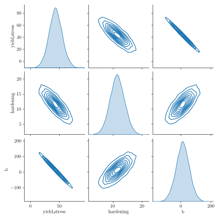
Next, we sample the multivariate normal provided by the study covariance and calibrated values as the mean and visualize the results using seaborn’s KDE pair plot

num_samples=5000
uncertain_param_sets = sample_multivariate_normal(num_samples,
                                                  results.mean.to_list(),
                                                  results.fitted_parameter_covariance,
                                                  12345,
                                                  pc.get_item_names())
import seaborn as sns
import pandas as pd
sns.pairplot(data=pd.DataFrame(uncertain_param_sets), kind="kde" )
plt.show()
# From this plot, we can see the uncertainty is considerably overestimated
# and could result in unphysical values of the parameters. This method is still
# work in progress for models with significant model form error.

/gpfs/knkarls/projects/matcal-stable/external_matcal/matcal/core/parameter_studies.py:919: RuntimeWarning: covariance is not symmetric positive-semidefinite.
  samples = rng.multivariate_normal(mean, sigma, nsamples).T