Top Hat Shear Model
MatCal’s TopHatShearModel
is meant to be used in calibrations requiring the simulation of the
Sandia developed top hat shear test where lower stress triaxialities are
required for parameter calibration (See [3] and [4]).
This model has all the MatCal standard
model features as described in MatCal SIERRA Solid Mechanics Standard Models.
In this section, we will provide more information about how the geometry is generated,
specifics on simulation boundary conditions,
and what is output from this model.
Note
Some examples and V&V studies that include these models are:
Top hat shear geometry and mesh generation
For the top hat geometry to be accurately built, the model requires the following keyword arguments be provided to its constructor.
total_height
base_height
hole_height
base_bottom_height
top_width
base_width
lower_radius_center_width
thickness
external_radius
internal_radius
trapezoid_angle
element_size
numsplits
localization_region_scale
These parameters provide information related to geometry, discretization sizing and output and boundary condition mesh entities such as blocks and node sets. The geometric parameters are shown in Fig. 12.
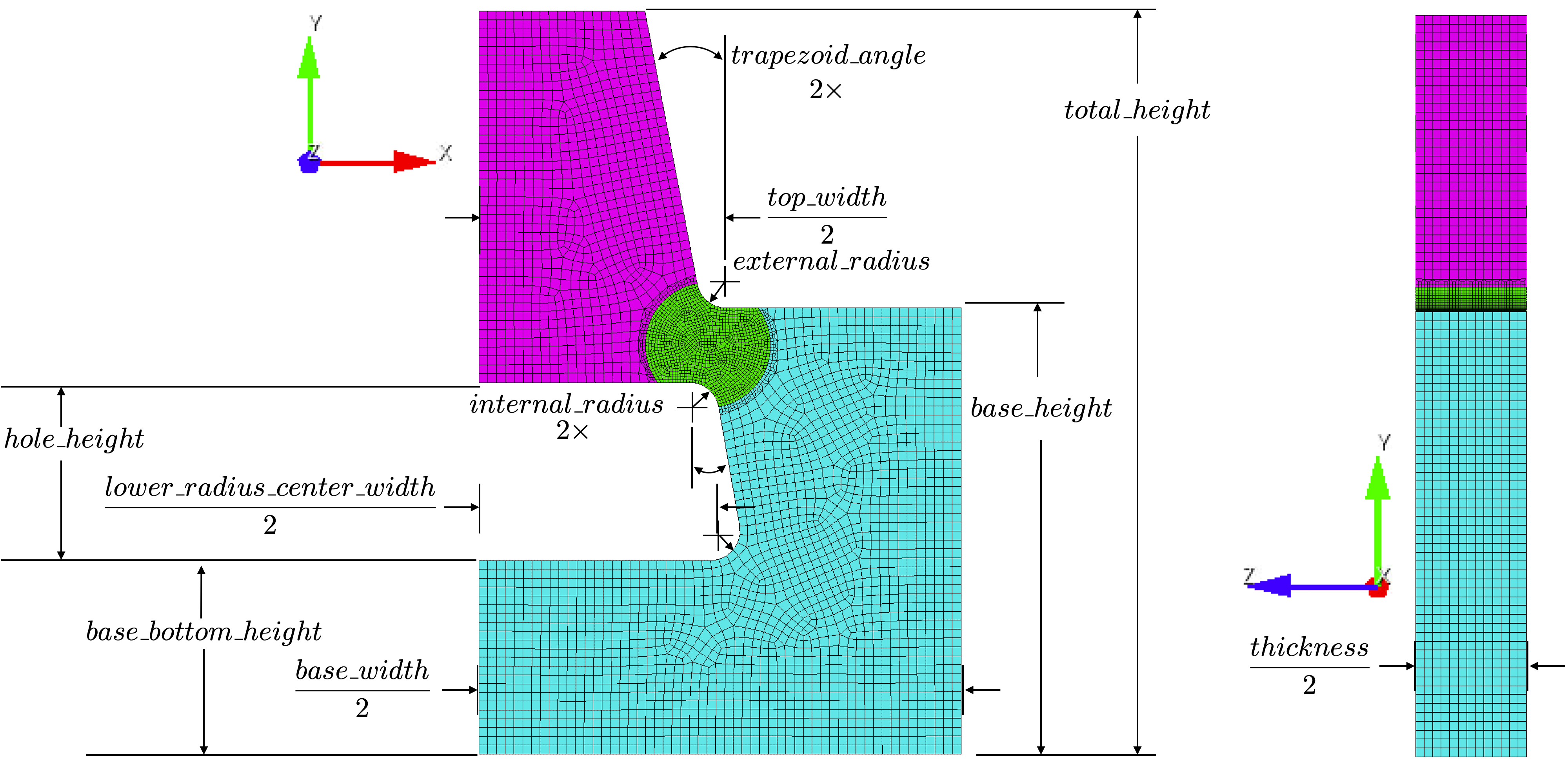
Fig. 12 The geometric dimensions for the top_hat_shear model.
The keyword element_size is used to specify the approximate element edge length that Cubit will target in the mesh. Depending on the number of numsplits specified, this could be the entire model or just a subregion of the model. The numsplits parameter allows the user to change how the geometry is around the localization region block is meshed. The localization region block and the effect of numsplits is shown in Fig. 13. The localization region should be more finely meshed since the deformation for this test is localized to the shear bands that form in this region. As a result, it is recommended to use at least numsplits = 1. Note that the numsplits parameter cannot be greater than 2 due to the poor quality elements created at the numpslit surface and the very low refinement away from the localization region.
By default, the geometry is made such that the localization region
is a cylinder centered between the farthest vertical locations in the two radius transitions
near the localization region. The radius of the cylinder is set so that it intersects with the end of
these two radius transitions.
The size of the localization region
can be modified using the localization_region_scale parameter.
This parameter increases the localization region by adding
 to
this radius. Essentially, the cylinder radius is scaled by an addition of some fraction of
the far field mesh size to it. As a result, it is recommended that integers be used
for this parameter, although, that is not required.
to
this radius. Essentially, the cylinder radius is scaled by an addition of some fraction of
the far field mesh size to it. As a result, it is recommended that integers be used
for this parameter, although, that is not required.
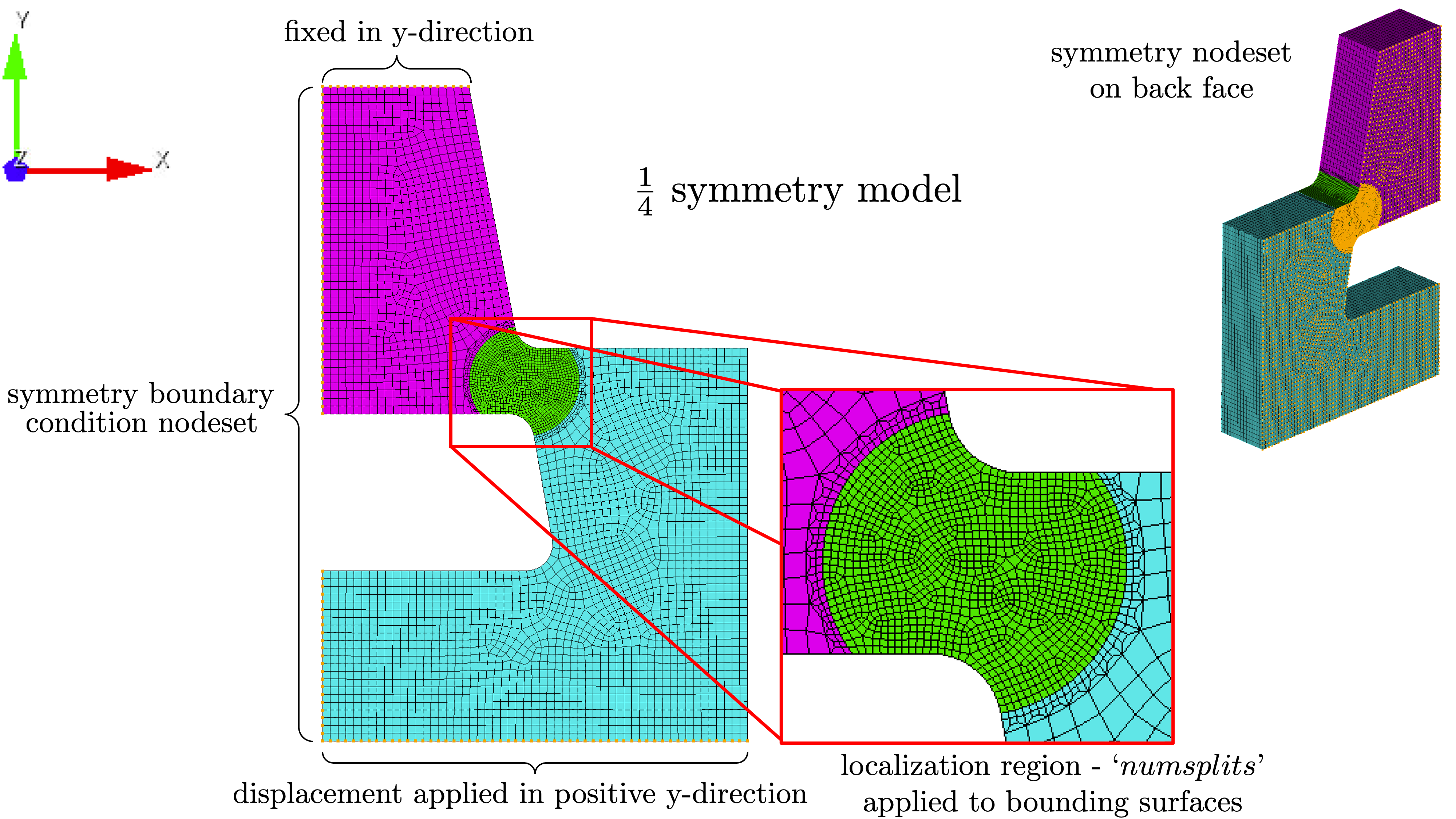
Fig. 13 The boundary condition nodesets for the top hat shear model and a resulting mesh with numsplits = 1.
Top hat shear boundary conditions
This model currently only supports  symmetry geometry,
and, as a result, has boundary conditions that reflect that. The boundary
condition nodesets are shown in Fig. 7.
Since this model can easily be coupled with thermal modeling, the boundary condition
descriptions have been separated into the following two subsections
associated with the solid mechanics and thermal models.
symmetry geometry,
and, as a result, has boundary conditions that reflect that. The boundary
condition nodesets are shown in Fig. 7.
Since this model can easily be coupled with thermal modeling, the boundary condition
descriptions have been separated into the following two subsections
associated with the solid mechanics and thermal models.
Top hat shear solid mechanics boundary conditions
The shear band in the localization region is caused by a displacement function
applied to the lower surface
of the top hat geometry applied in the vertical y-direction.
This function acts on the surface of the specimen
where the platens would contact it.
The applied function is determined using the
add_boundary_condition_data().
This method must be supplied a Data or
DataCollection class that contains
at a “displacement” field for the
states of interest for the model. They can also optionally include
a “time” field. The
add_boundary_condition_data()
method determines the boundary condition function to be applied
to the specimen according to the following
algorithm:
Determine the boundary condition by state since maximum deformation, material behavior and experiment setup can vary significantly over different states.
For each state, find the data set with the largest displacement and use it for boundary condition generation.
Perform no scaling on the displacement. This assumes that the strain is primarily localized to the notched region of the specimen.
If the data does not contain a “time” field and there is not a
Stateparameter named “displacement_rate”, then apply a linear displacement function from zero to the maximum displacement found in the data over one second.If the data does not contain a “time” field and there is a
Stateparameter named “displacement_rate”, then apply a linear displacement function from zero to the maximum displacement found in the data. This is done over a time period beginning at zero seconds and ending at a time calculated by dividing the maximum displacement at the extensometer by the “displacement_rate”Stateparameter.If the data does contain a “time” field, use the displacement function directly as provided.
The remaining solid mechanics boundary conditions only include the symmetry boundary conditions where displacements normal to the symmetry surfaces are set to zero.
Top hat shear thermal model boundary conditions
Since MatCal SIERRA/SM standard models only allow
heat flux out of the specimen through the platens,
only the platen contact boundary condition is
described here. The boundary condition for the
platen-to-specimen interface
includes the nodes at the top and bottom of the top
hat specimen.
As described in Staggered and iterative coupling,
the temperature at the nodes is fixed to the value of the State parameter
“temperature”. The entire body
of the model is prescribed an initial temperate of
State parameter
“temperature” for
all simulations regardless of coupling specification (uncoupled, staggered coupling,
iterative coupling or adiabatic). For uncoupled simulations, this is only done
if a temperature state variable is provided.
Top hat shear model specific output
By default, the top hat shear model includes the following global output fields:
time
displacement - measured across extensometer length in the loading direction
load - measured at the applied boundary condition node set in the loading direction.
If coupling is activated, the following global temperature output is provided:
low_temperature
med_temperature
high_temperature
and how they are calculated is dependent on the type of coupling. For adiabatic simulations, they are the minimum, average and maximum element temperatures in the gauge section of the model. For coupled simulations, the same quantities are provided by acting on the nodal temperatures instead of the element temperatures.