Solid Bar Torsion Model

MatCal’s SolidBarTorsionModel is meant to be used in calibrations requiring the simulation of the Sandia developed solid bar torsion test where lower stress triaxialities are required for parameter calibration (See [16]). This model has all the MatCal standard model features as described in MatCal SIERRA Solid Mechanics Standard Models. In this section, we will provide more information about how the geometry is generated, specifics on simulation boundary conditions, and what is output from this model.

Note

Some examples and V&V studies that include these models are:

1. Comparing iterative, staggered and adiabatic coupling solutions

Solid bar torsion geometry and mesh generation

The solid bar torsion geometry uses the same mesh generation script as is used by the RoundUniaxialTensionModel and requires the input for that model specified in Uniaxial Tension Models. All inputs and behavior for meshing are the same except that the geometry produced is half of the model. The model is split at the specimen center along the specimen axis with a plane that has its normal aligned with the specimen axis.

Solid bar torsion boundary conditions

This model currently only includes of the specimen geometry, with antisymmetric solid mechanics boundary conditions at the specimen axial midplane. The boundary condition nodesets are shown in Fig. 10.

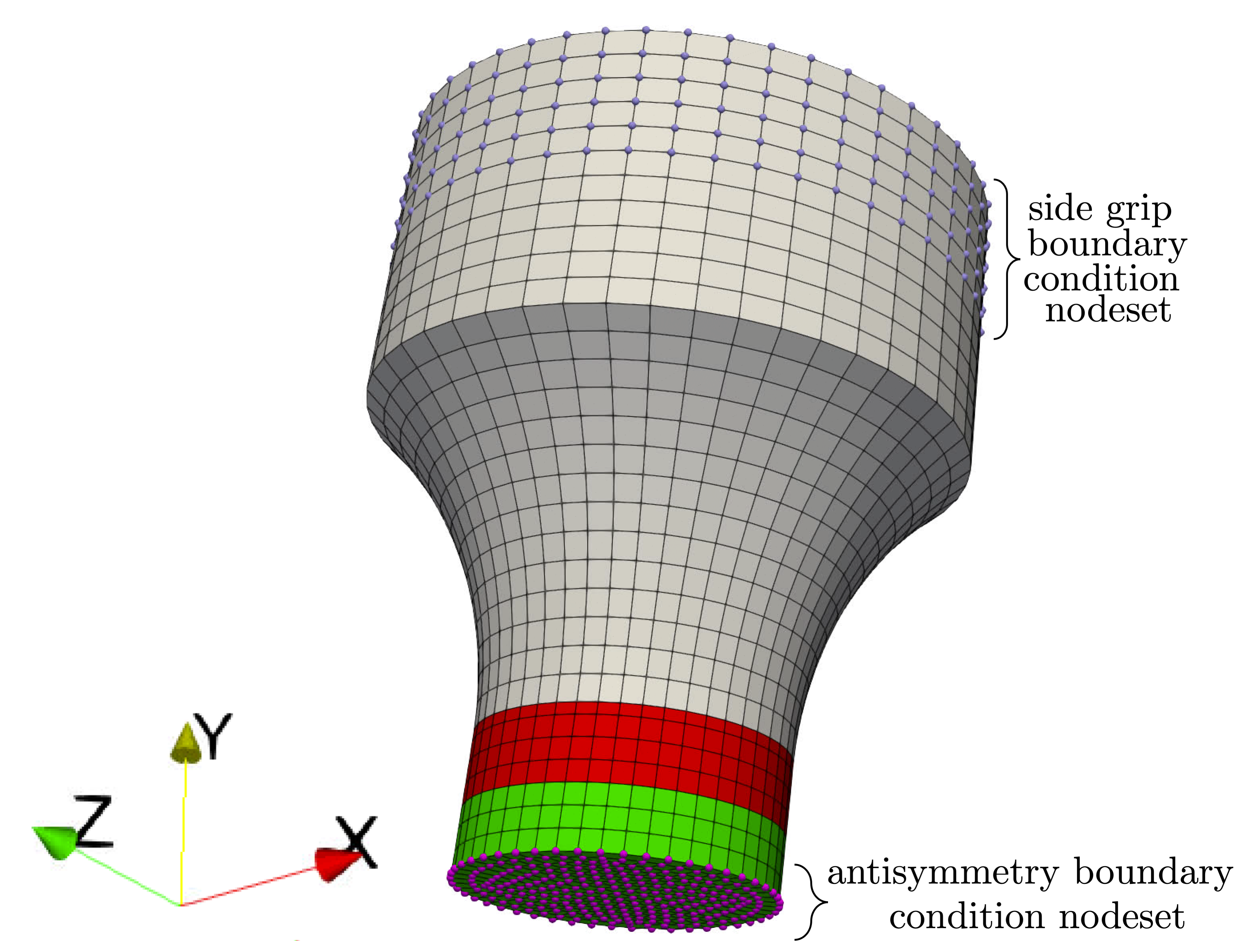
Fig. 10 The boundary condition node sets for this model are shown on its mesh. Two node sets are important, the side grip node set and the antisymmetry node set at the specimen midplane.

Since this model can easily be coupled with thermal modeling, the boundary condition descriptions have been separated into the following two subsections associated with the solid mechanics and thermal models.

Solid bar torsion solid mechanics boundary conditions

The model is deformed with a rotation applied to the side grip node set. Positive rotations are applied around the specimen axis (aligned with the global Y axis) according to the right hand rule. The applied rotation function is determined using the add_boundary_condition_data(). This method must be supplied a Data or DataCollection class that contains a “grip_rotation” field for the states of interest for the model with units of degrees. The boundary condition data can also optionally include a “time” field. The add_boundary_condition_data() method determines the boundary condition function to be applied to the specimen according to the following algorithm:

1. Determine the boundary condition by state since maximum deformation, material behavior and experiment setup can vary significantly over different states.

2. For each state, find the data set with the largest rotation and use it for boundary condition generation.

3. Perform no scaling on the rotation. This assumes that the deformation is primarily localized to the gauge section region of the specimen.

4. If the data do not contain a “time” field and there is not a State parameter named “rotation_rate”, then apply a linear rotation function from zero to the maximum rotation found in the data over one second.

5. If the data do not contain a “time” field and there is a State parameter named “rotation_rate”, then apply a linear rotation function from zero to the maximum rotation found in the data. This is done over a time period beginning at zero seconds and ending at a time calculated by dividing the maximum rotation by the “rotation_rate” State parameter.

6. If the data do contain a “time” field, use the rotation function directly as provided.

The remaining solid mechanics boundary conditions only include the antisymmetry boundary condition at the specimen midplane where the displacements are fixed around the specimen axis and normal to the mid plane. At this midplane, the nodes are allowed to displace in the radial direction only.

Solid bar torsion thermal model boundary conditions

Since MatCal SIERRA/SM standard models only allow heat flux out of the specimen through the model’s interface at the grips, only the grip contact boundary condition is described here. The boundary condition for the grip-to-specimen interface includes the nodes in the side grip node set. As described in Staggered and iterative coupling, the temperature at these nodes is fixed to the value of the State parameter “temperature”. The entire body of the model is prescribed an initial temperature of State parameter “temperature” for all simulations regardless of coupling specification (uncoupled, staggered coupling, iterative coupling or adiabatic). For uncoupled simulations, this is only done if a temperature state variable is provided.

Solid bar torsion model specific output

By default, the solid bar torsion model includes the following global output fields:

1. time

2. applied_rotation - the rotation in degrees determined from the boundary condition data set

3. grip_rotation - the rotation in degrees measured at the applied boundary condition node set in the loading direction.

4. torque - measured at the applied boundary condition node set in the loading direction

If coupling is activated, the following global temperature output is provided:

1. low_temperature

2. med_temperature

3. high_temperature

and how they are calculated is dependent on the type of coupling. For adiabatic simulations, they are the minimum, average and maximum element temperatures in the gauge section of the model. For coupled simulations, the same quantities are provided by acting on the nodal temperatures instead of the element temperatures.

The model also includes torsion specific exodus output that the user can output if desired. Two nodal variables are available for exodus output, cylindrical_displacement and cylindrical_force_external. To add these to the exodus output, you must call the activate_exodus_output() method and then add them to output using the add_nodal_output_variable() method. These variables are transformed to the cylindrical_coordinate_system described in Simulation Coordinate Systems Available to the Material Model. As a result, these nodal variables are defined in a local Cartesian coordinate system defined at each node in the model’s deformed configuration. As an example, a drawing of the local coordinate system displacements on a cylinder is shown in Fig. 11.

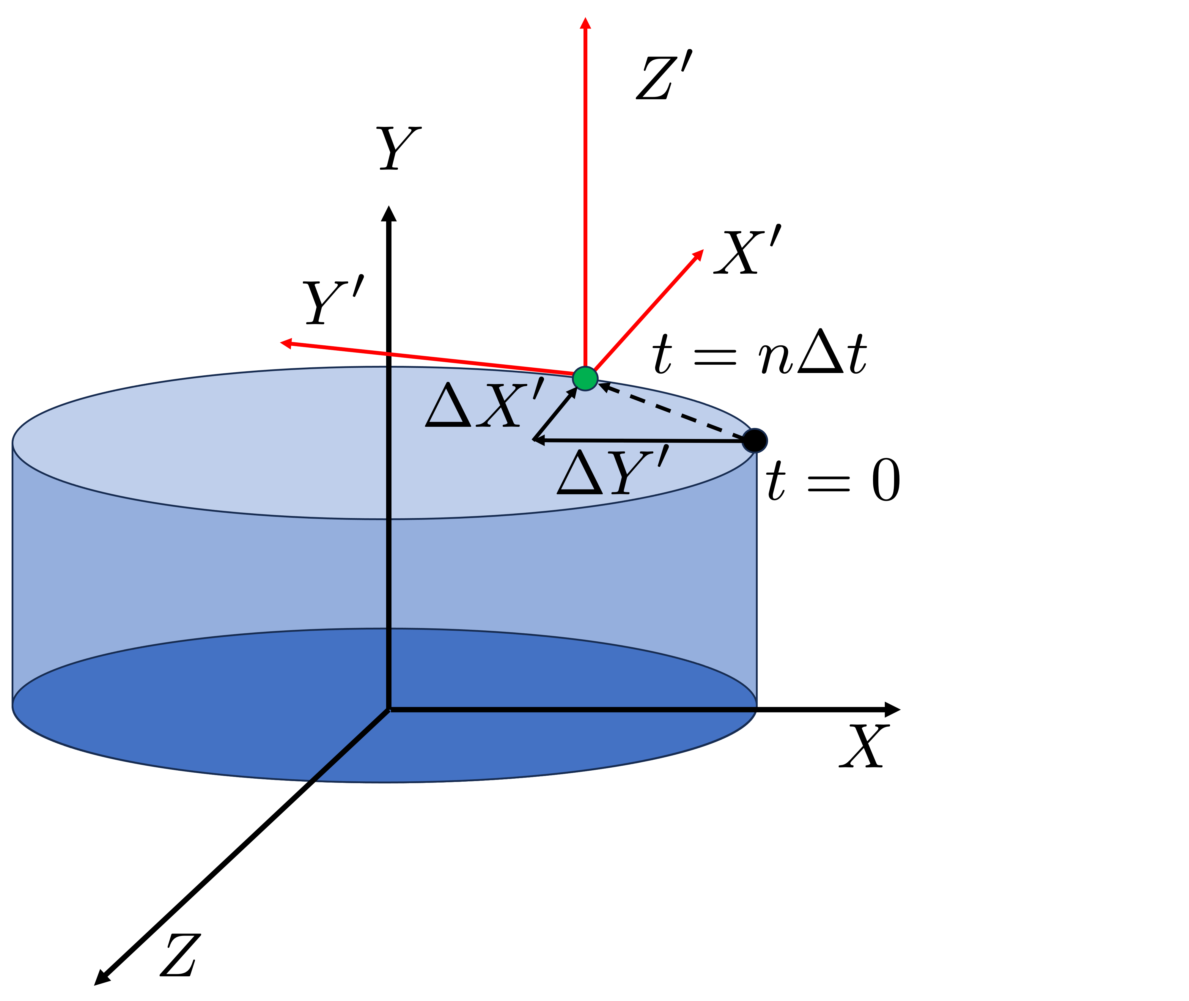
Fig. 11 A diagram showing the displacement of a point at in the cylindrical_coordinate_system local coordinate system. The local coordinate system is defined in the model’s deformed configuration.