Note
Go to the end to download the full example code.
Comparing iterative, staggered and adiabatic coupling solutions
Note
Useful Documentation links:
As discussed in Uniaxial Tension Models, three coupling options are available in MatCal when using MatCal standard models. The easiest to use is adiabatic coupling which relies primarily on the SIERRA/SM material model to handle the temperature evolution due to heating due to plastic work. The adiabatic coupling feature is well verified in LAME and SIERRA/SM [27, 34]. The other two methods, staggered and iterative coupling, rely on the MatCal generated input to properly setup the coupling schemes. In MatCal, we define staggered coupling as two-way coupling where first the solid mechanics solution is updated in a time step, the displacements and plastic work from the solid mechanics solution is passed to the thermal model, the updated temperature is calculated from the thermal model solve, and, finally, the temperatures are passed to the solid mechanics model to finish the time step. There is no iteration on the staggered scheme. For the iterative coupling scheme, the staggered scheme is repeated until the initial thermal model residual is below some threshold.
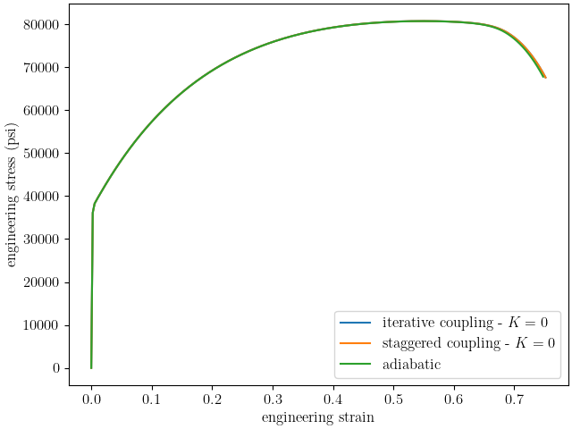
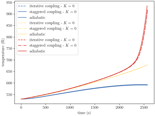
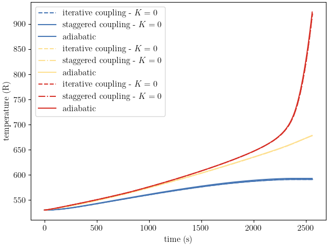
To verify our SIERRA input for these coupling methods, we compare engineering stress-strain curves, temperature histories and objective values for the three different coupling methods applied to the same model. For the iterative and staggered coupling methods, we will set the material thermal conductivity to zero so that they will also be modeling the adiabatic condition. Since adiabatic coupling is well verified, we use it as the reference to which the iterative and staggered solutions will be compared. This example is an extension of the 304L annealed bar viscoplastic calibrations examples. We use the calibrated parameters, the study setup and the converged discretizations from that set of examples here. We then verify that the MatCal generated models produce the correct responses for the different coupling options. We also perform a simple time step convergence study on the model results to see the effect of improved time resolution.
To begin, we once again perform the data import, model preparation and objective specification for the tension model from the examples linked above.
from matcal import *
import matplotlib.pyplot as plt

plt.rc('text', usetex=True)
plt.rc('font', family='serif')
plt.rc('font', size=12)
figsize = (4,3)


data_collection = BatchDataImporter("ductile_failure_ASTME8_304L_data/*.dat", file_type="csv")
data_collection.set_fixed_state_parameters(displacement_rate=2e-4, temperature=530)
data_collection = data_collection.batch
data_collection = scale_data_collection(data_collection, "engineering_stress", 1000)
data_collection.remove_field("time")

yield_stress = Parameter("Y_0", 30, 40, 35)
A = Parameter("A", 100, 300, 200)
b = Parameter("b", 0, 3, 2.0)
C = Parameter("C", -3, -1)

sierra_material = Material("304L_viscoplastic", "304L_viscoplastic_voce_hardening.inc",
                           "j2_plasticity")

geo_params = {"extensometer_length": 0.75,
               "gauge_length": 1.25,
               "gauge_radius": 0.125,
               "grip_radius": 0.25,
               "total_length": 4,
               "fillet_radius": 0.188,
               "taper": 0.0015,
               "necking_region":0.375,
               "element_size": 0.005,
               "mesh_method":4,
               "grip_contact_length":1}

staggered_coupling = RoundUniaxialTensionModel(sierra_material, **geo_params)
staggered_coupling.add_boundary_condition_data(data_collection)
from site_matcal.sandia.computing_platforms import is_sandia_cluster, get_sandia_computing_platform
from site_matcal.sandia.tests.utilities import MATCAL_WCID

num_cores = 24
if is_sandia_cluster():
    platform = get_sandia_computing_platform()
    num_cores = platform.processors_per_node
    staggered_coupling.run_in_queue(MATCAL_WCID, 4)
    staggered_coupling.continue_when_simulation_fails()
staggered_coupling.set_number_of_cores(num_cores)
staggered_coupling.add_constants(ref_strain_rate=1e-5, coupling="coupled",
                                      density=0.000741,
                                      specific_heat=4.13e+05)
staggered_coupling.set_allowable_load_drop_factor(0.15)
staggered_coupling.activate_thermal_coupling(thermal_conductivity=0.0,
                                      density=0.000741,
                                      specific_heat=4.13e+05,
                                      plastic_work_variable="plastic_work_heat_rate")
staggered_coupling.set_name("ASTME8_tension_model_staggered_coupling")

objective = CurveBasedInterpolatedObjective("engineering_strain", "engineering_stress")
objective.set_name("stress_objective")
Now to setup the different coupling models, we will use Python’s copy
module to copy the astme8_model_staggered_coupling model, and the set
the correct coupling options
for the new models.
from copy import deepcopy
iterative_coupling = deepcopy(staggered_coupling)
iterative_coupling.set_name("ASTME8_tension_model_iterative_coupling")
iterative_coupling.use_iterative_coupling()

adiabatic = RoundUniaxialTensionModel(sierra_material, **geo_params)
adiabatic.add_boundary_condition_data(data_collection)
adiabatic.set_name("ASTME8_tension_model_adiabatic")
if is_sandia_cluster():
    adiabatic.run_in_queue(MATCAL_WCID, 4)
    adiabatic.continue_when_simulation_fails()
adiabatic.set_number_of_cores(num_cores)
adiabatic.add_constants(ref_strain_rate=1e-5, coupling="adiabatic", density=0.000741,
                                      specific_heat=4.13e+05)
adiabatic.set_allowable_load_drop_factor(0.15)
adiabatic.activate_thermal_coupling()
Similar to what was done in the convergence study,
we will perform a ParameterStudy
where the only parameters
to be evaluated are the calibrated parameters from the initial study.
We then add evaluation sets for each of the models with the different coupling
methods.
param_study = ParameterStudy(yield_stress, A, b, C)
calibrated_params = {"A": 159.62781358, "C": -1.3987056852,
                     "Y_0": 33.008981584, "b": 1.9465943453}
param_study.add_parameter_evaluation(**calibrated_params)
param_study.set_working_directory("coupling_study", remove_existing=True)
param_study.add_evaluation_set(staggered_coupling, objective, data_collection)
param_study.add_evaluation_set(iterative_coupling, objective, data_collection)
param_study.add_evaluation_set(adiabatic, objective, data_collection)
param_study.set_core_limit(112)
We can now run the study, and after it finishes, we can compare the results from the different models. For our purposes, we want to ensure that the objective value is the same for each model or has an acceptable error. As a result, we manipulate the results output from this study to access the objective values for each model, and then use Matplotlib [9] to plot the raw simulation stress-strain and temperature-time curves.
Since we will repeat the results manipulation for repeated studies where these models have more time steps, we put it into a function that can be called on each of the additional study results. This function plots the desired simulation results curves, and it also returns the different models’ objectives and number of time steps taken during the simulation. We will use this data to plot time step convergence plots for the objective once all the simulations are completed.
results = param_study.launch()
state = data_collection.state_names[0]
def get_and_plot_results(results):
    iterative_coupling_objective = results.best_evaluation_set_objective(iterative_coupling, objective)
    iterative_coupling_curves = results.best_simulation_data(iterative_coupling, state)

    staggered_coupling_objective = results.best_evaluation_set_objective(staggered_coupling, objective)
    staggered_coupling_curves = results.best_simulation_data(staggered_coupling, state)

    adiabatic_objective = results.best_evaluation_set_objective(adiabatic, objective)
    adiabatic_curves = results.best_simulation_data(adiabatic, state)

    plt.figure(constrained_layout=True)
    plt.plot(iterative_coupling_curves["engineering_strain"], iterative_coupling_curves["engineering_stress"], label="iterative coupling - $K=0$")
    plt.plot(staggered_coupling_curves["engineering_strain"], staggered_coupling_curves["engineering_stress"], label="staggered coupling - $K=0$")
    plt.plot(adiabatic_curves["engineering_strain"], adiabatic_curves["engineering_stress"], label="adiabatic")
    plt.xlabel("engineering strain")
    plt.ylabel("engineering stress (psi)")
    plt.legend()

    plt.figure(constrained_layout=True)
    plt.plot(iterative_coupling_curves["time"], iterative_coupling_curves["low_temperature"], '--', color="#4575b4", label="iterative coupling - $K=0$")
    plt.plot(staggered_coupling_curves["time"], staggered_coupling_curves["low_temperature"], color="#4575b4", label="staggered coupling - $K=0$")
    plt.plot(adiabatic_curves["time"], adiabatic_curves["low_temperature"], color="#4575b4", label="adiabatic")

    plt.plot(iterative_coupling_curves["time"], iterative_coupling_curves["med_temperature"],  '--', color="#fee090", label="iterative coupling - $K=0$")
    plt.plot(staggered_coupling_curves["time"], staggered_coupling_curves["med_temperature"], '-.', color="#fee090", label="staggered coupling - $K=0$")
    plt.plot(adiabatic_curves["time"], adiabatic_curves["med_temperature"], color="#fee090", label="adiabatic")

    plt.plot(iterative_coupling_curves["time"], iterative_coupling_curves["high_temperature"],  '--', color="#d73027", label="iterative coupling - $K=0$")
    plt.plot(staggered_coupling_curves["time"], staggered_coupling_curves["high_temperature"], '-.', color="#d73027", label="staggered coupling - $K=0$")
    plt.plot(adiabatic_curves["time"], adiabatic_curves["high_temperature"], color="#d73027", label="adiabatic")

    plt.xlabel("time (s)")
    plt.ylabel("temperature (R)")

    plt.legend()

    objective_results = [iterative_coupling_objective,
                         staggered_coupling_objective,
                         adiabatic_objective,
                         len(iterative_coupling_curves["time"]),
                         len(staggered_coupling_curves["time"]),
                         len(adiabatic_curves["time"])]

    return objective_results

coarse_objective_results = get_and_plot_results(results)
iterative_objective_coarse = coarse_objective_results[0]
staggered_objective_coarse = coarse_objective_results[1]
adiabatic_objective_coarse = coarse_objective_results[2]
iterative_coarse_time_steps = coarse_objective_results[3]
staggered_coarse_time_steps = coarse_objective_results[4]
adiabatic_coarse_time_steps = coarse_objective_results[5]
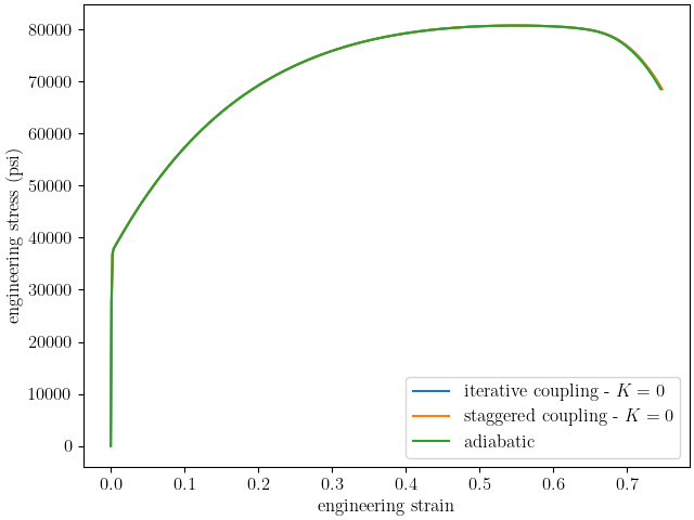
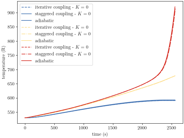
We now update the time steps for each model, and then we create a new study for the updated model. The new study is launched and the results are once again plotted and stored for the objective time step convergence plot.
staggered_coupling.set_number_of_time_steps(600)
iterative_coupling.set_number_of_time_steps(600)
adiabatic.set_number_of_time_steps(600)

param_study = ParameterStudy(yield_stress, A, b, C)
param_study.add_parameter_evaluation(**calibrated_params)
param_study.add_evaluation_set(staggered_coupling, objective, data_collection)
param_study.add_evaluation_set(iterative_coupling, objective, data_collection)
param_study.add_evaluation_set(adiabatic, objective, data_collection)
param_study.set_core_limit(112)

results = param_study.launch()

med_objective_results = get_and_plot_results(results)
iterative_objective_med = med_objective_results[0]
staggered_objective_med = med_objective_results[1]
adiabatic_objective_med = med_objective_results[2]
iterative_med_time_steps = med_objective_results[3]
staggered_med_time_steps = med_objective_results[4]
adiabatic_med_time_steps = med_objective_results[5]
This process is completed one last time for models with a target of 1200 time steps for their simulations.
staggered_coupling.set_number_of_time_steps(1200)
iterative_coupling.set_number_of_time_steps(1200)
adiabatic.set_number_of_time_steps(1200)

param_study = ParameterStudy(yield_stress, A, b, C)
param_study.add_parameter_evaluation(**calibrated_params)
param_study.add_evaluation_set(staggered_coupling, objective, data_collection)
param_study.add_evaluation_set(iterative_coupling, objective, data_collection)
param_study.add_evaluation_set(adiabatic, objective, data_collection)
param_study.set_core_limit(112)

results = param_study.launch()

fine_objective_results = get_and_plot_results(results)
iterative_objective_fine = fine_objective_results[0]
staggered_objective_fine = fine_objective_results[1]
adiabatic_objective_fine = fine_objective_results[2]
iterative_fine_time_steps = fine_objective_results[3]
staggered_fine_time_steps = fine_objective_results[4]
adiabatic_fine_time_steps = fine_objective_results[5]

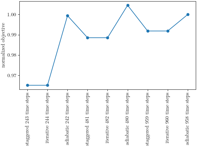
With all objective results complete, we can plot the objectives for each model as a function of time step and coupling method. The goal is to see whether the objectives are converging to a common value.
plt.figure(constrained_layout=True)
import numpy as np
objectives = np.array([staggered_objective_coarse, iterative_objective_coarse, adiabatic_objective_coarse,
          staggered_objective_med, iterative_objective_med, adiabatic_objective_med,
          staggered_objective_fine, iterative_objective_fine, adiabatic_objective_fine,])
x_pos = np.arange(len(objectives))

plt.plot(x_pos,
         objectives/adiabatic_objective_fine, 'o-')
xtick_lables = [f"staggered {staggered_coarse_time_steps} time steps",
                f"iterative {iterative_coarse_time_steps} time steps",
                f"adiabatic {adiabatic_coarse_time_steps} time steps",
                f"staggered {staggered_med_time_steps} time steps",
                f"iterative {iterative_med_time_steps} time steps",
                f"adiabatic {adiabatic_med_time_steps} time steps",
                f"staggered {staggered_fine_time_steps} time steps",
                f"iterative {iterative_fine_time_steps} time steps",
                f"adiabatic {adiabatic_fine_time_steps} time steps",
                ]

plt.xticks(x_pos, xtick_lables,rotation=90 )
plt.ylabel("normalized objective")

plt.show()
/gpfs/knkarls/projects/matcal_devel/external_matcal/documentation/matcal_model_v_and_v/plot_coupling_verification.py:295: RuntimeWarning: invalid value encountered in divide
  objectives/adiabatic_objective_fine, 'o-')
The results displayed in the plots are notable and indicate that the coupling models may need improvement. Although it is clear that the objectives, engineering stress-strain curves and temperature-time curves are converging as the number of time steps increase, the convergence is rather slow. However, the results exhibit relatively low error, and the models are useful for intermediate rates where they will be used. With about 900 time steps, the objective errors for the coupled models are on the order of 1% for this study when compared to the adiabatic model. Any errors introduced by the coupling scheme are expected to have less of an effect for simulations with conduction within the material because the overall increase in temperature and, therefore, the structural softening due to temperature will be reduced. As a result, the iterative and staggered coupling models are considered accurate for user calibrations. We are actively working with the SIERRA developers to identify and correct any issues and will update the models if an issue is found and resolved.
Total running time of the script: (109 minutes 51.053 seconds)