Effect of mesh_method on simulation results

Note

Useful Documentation links:

1. Uniaxial Tension Models

2. RoundUniaxialTensionModel

3. ObjectiveResults

4. ParameterStudy

5. 304L annealed bar viscoplastic calibrations

As discussed in Uniaxial Tension Models, several meshing options are available in MatCal when using these models. Since changing the meshing scheme can result in small changes to the results, we compare the engineering stress-strain curves and objective values for all meshing methods applied to the same model for a common target element size of 0.0035.

Note

This size is chosen so that all meshing schemes can be used since some methods have restrictions on what element size can be used. These limits are a function of element size relative to the gauge radius.

This example is an extension of the 304L annealed bar viscoplastic calibrations examples. We use the calibrated parameters and the study setup from that set of examples here. We then quantify the changes to the model outputs based on mesh_method choice.

To begin, we once again perform the data import, model preparation and objective specification for the tension model from the example linked above.

from matcal import *
import matplotlib.pyplot as plt

plt.rc('text', usetex=True)
plt.rc('font', family='serif')
plt.rc('font', size=12)
figsize = (4,3)

data_collection = BatchDataImporter("ductile_failure_ASTME8_304L_data/*.dat", file_type="csv")
data_collection.set_fixed_state_parameters(displacement_rate=2e-4, temperature=530)
data_collection = data_collection.batch
data_collection = scale_data_collection(data_collection, "engineering_stress", 1000)
data_collection.remove_field("time")

yield_stress = Parameter("Y_0", 30, 40, 35)
A = Parameter("A", 100, 300, 200)
b = Parameter("b", 0, 3, 2.0)
C = Parameter("C", -3, -1)


sierra_material = Material("304L_viscoplastic", "304L_viscoplastic_voce_hardening.inc",
                           "j2_plasticity")

geo_params = {"extensometer_length": 0.75,
               "gauge_length": 1.25,
               "gauge_radius": 0.125,
               "grip_radius": 0.25,
               "total_length": 4,
               "fillet_radius": 0.188,
               "taper": 0.0015,
               "necking_region":0.375,
               "element_size": 0.125/36,
               "mesh_method":1,
               "grip_contact_length":1}

mesh_method_1 = RoundUniaxialTensionModel(sierra_material, **geo_params)
mesh_method_1.add_boundary_condition_data(data_collection)
from site_matcal.sandia.computing_platforms import is_sandia_cluster, get_sandia_computing_platform
from site_matcal.sandia.tests.utilities import MATCAL_WCID

num_cores = 24
mesh_method_1.set_number_of_cores(num_cores)
if is_sandia_cluster():
    platform = get_sandia_computing_platform()
    num_cores = platform.processors_per_node
    mesh_method_1.run_in_queue(MATCAL_WCID, 4)
    mesh_method_1.continue_when_simulation_fails()
    mesh_method_1.set_number_of_cores(num_cores*4)
mesh_method_1.set_allowable_load_drop_factor(0.15)
mesh_method_1.set_name("ASTME8_tension_model_mesh_method_1")
mesh_method_1.add_constants(ref_strain_rate=1e-5, coupling="coupled")

objective = CurveBasedInterpolatedObjective("engineering_strain", "engineering_stress")
objective.set_name("stress_objective")

def remove_uncalibrated_data_from_residual(engineering_strains, engineering_stresses, residuals):
    import numpy as np
    weights = np.ones(len(residuals))
    weights[engineering_stresses < 38e3] = 0
    weights[engineering_strains > 0.75] = 0
    return weights*residuals

residual_weights = UserFunctionWeighting("engineering_strain", "engineering_stress", remove_uncalibrated_data_from_residual)
objective.set_field_weights(residual_weights)

Now to setup the mesh_method study, we will use Python’s copy module to copy the astme8_model_mesh_method_1 model and modify the mesh_method geometry parameter for the new models. This can be done with the add_constants() method which can be used to override geometry parameters if desired. We also change the number of cores to be used for each model because the higher mesh_method schemes result in fewer elements being created for the meshed geometry.

from copy import deepcopy
mesh_method_2 = deepcopy(mesh_method_1)
mesh_method_2.add_constants(mesh_method=2)
mesh_method_2.set_name("ASTME8_tension_model_mesh_method_2")

mesh_method_3 = deepcopy(mesh_method_1)
mesh_method_3.add_constants(mesh_method=3)
if is_sandia_cluster():
    mesh_method_3.set_number_of_cores(num_cores*3)
mesh_method_3.set_name("ASTME8_tension_model_mesh_method_3")

mesh_method_4 = deepcopy(mesh_method_1)
mesh_method_4.add_constants(mesh_method=4)
if is_sandia_cluster():
    mesh_method_4.set_number_of_cores(num_cores*2)
mesh_method_4.set_name("ASTME8_tension_model_mesh_method_4")

mesh_method_5 = deepcopy(mesh_method_1)
mesh_method_5.add_constants(mesh_method=5)
if is_sandia_cluster():
    mesh_method_5.set_number_of_cores(num_cores)
mesh_method_5.set_name("ASTME8_tension_model_mesh_method_5")

Once again, we will perform a ParameterStudy where the only parameters to be evaluated are the calibrated parameters from the initial study. This mesh_method study will need to evaluate all models we created, so each is added to the study as their own evaluation set. Lastly, the study core limit is set appropriately.

param_collection = ParameterCollection("my_parameters", yield_stress, A, b, C)
calibrated_params = {"A": 159.62781358, "C": -1.3987056852,
                     "Y_0": 33.008981584, "b": 1.9465943453}
param_collection.update_parameters(**calibrated_params)
param_study = ParameterStudy(param_collection)
param_study.set_working_directory("mesh_method_study", remove_existing=True)
param_study.add_evaluation_set(mesh_method_1, objective, data_collection)
param_study.add_evaluation_set(mesh_method_2, objective, data_collection)
param_study.add_evaluation_set(mesh_method_3, objective, data_collection)
param_study.add_evaluation_set(mesh_method_4, objective, data_collection)
param_study.add_evaluation_set(mesh_method_5, objective, data_collection)
param_study.set_core_limit(112)

param_study.add_parameter_evaluation(**calibrated_params)

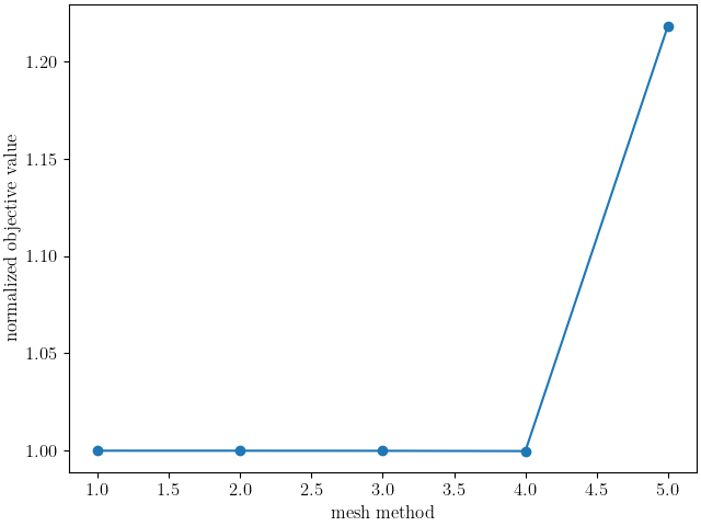
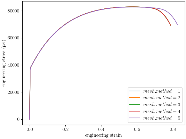
We can now run the study. After it finishes, we can make our results plots. We manipulate the results output from this study to access the objective values for each mesh_method. We then use Matplotlib [9] to plot the values versus the different mesh_method options numbers. We also plot the raw simulation stress-strain curves.

results = param_study.launch()

state = data_collection.state_names[0]
mesh_method_1_objective_results = results.best_evaluation_set_objective(mesh_method_1, objective)
mesh_method_1_curves = results.best_simulation_data(mesh_method_1, state)

mesh_method_2_objective_results = results.best_evaluation_set_objective(mesh_method_2, objective)
mesh_method_2_curves = results.best_simulation_data(mesh_method_2, state)

mesh_method_3_objective_results = results.best_evaluation_set_objective(mesh_method_3, objective)
mesh_method_3_curves = results.best_simulation_data(mesh_method_3, state)

mesh_method_4_objective_results = results.best_evaluation_set_objective(mesh_method_4, objective)
mesh_method_4_curves = results.best_simulation_data(mesh_method_4, state)

mesh_method_5_objective_results = results.best_evaluation_set_objective(mesh_method_5, objective)
mesh_method_5_curves = results.best_simulation_data(mesh_method_5, state)

import matplotlib.pyplot as plt
import numpy as np

methods = [1, 2, 3, 4, 5]
objectives = np.array([mesh_method_1_objective_results,
                       mesh_method_2_objective_results,
                       mesh_method_3_objective_results,
                       mesh_method_4_objective_results,
                       mesh_method_5_objective_results])
plt.figure(constrained_layout=True)
plt.plot(methods, objectives/mesh_method_1_objective_results, 'o-')
plt.xlabel("mesh method")
plt.ylabel("normalized objective value")

plt.figure(constrained_layout=True)
plt.plot(mesh_method_1_curves["engineering_strain"], mesh_method_1_curves["engineering_stress"], label="$mesh\_method = 1$")
plt.plot(mesh_method_2_curves["engineering_strain"], mesh_method_2_curves["engineering_stress"], label="$mesh\_method = 2$")
plt.plot(mesh_method_3_curves["engineering_strain"], mesh_method_3_curves["engineering_stress"], label="$mesh\_method = 3$")
plt.plot(mesh_method_4_curves["engineering_strain"], mesh_method_4_curves["engineering_stress"], label="$mesh\_method = 4$")
plt.plot(mesh_method_5_curves["engineering_strain"], mesh_method_5_curves["engineering_stress"], label="$mesh\_method = 5$")
plt.xlabel("engineering strain")
plt.ylabel("engineering stress (psi)")
plt.legend()

• 
• 

/gpfs/knkarls/projects/matcal_devel/external_matcal/documentation/matcal_model_v_and_v/plot_round_tension_mesh_method_effects.py:202: SyntaxWarning: invalid escape sequence '\_'
  plt.plot(mesh_method_1_curves["engineering_strain"], mesh_method_1_curves["engineering_stress"], label="$mesh\_method = 1$")
/gpfs/knkarls/projects/matcal_devel/external_matcal/documentation/matcal_model_v_and_v/plot_round_tension_mesh_method_effects.py:203: SyntaxWarning: invalid escape sequence '\_'
  plt.plot(mesh_method_2_curves["engineering_strain"], mesh_method_2_curves["engineering_stress"], label="$mesh\_method = 2$")
/gpfs/knkarls/projects/matcal_devel/external_matcal/documentation/matcal_model_v_and_v/plot_round_tension_mesh_method_effects.py:204: SyntaxWarning: invalid escape sequence '\_'
  plt.plot(mesh_method_3_curves["engineering_strain"], mesh_method_3_curves["engineering_stress"], label="$mesh\_method = 3$")
/gpfs/knkarls/projects/matcal_devel/external_matcal/documentation/matcal_model_v_and_v/plot_round_tension_mesh_method_effects.py:205: SyntaxWarning: invalid escape sequence '\_'
  plt.plot(mesh_method_4_curves["engineering_strain"], mesh_method_4_curves["engineering_stress"], label="$mesh\_method = 4$")
/gpfs/knkarls/projects/matcal_devel/external_matcal/documentation/matcal_model_v_and_v/plot_round_tension_mesh_method_effects.py:206: SyntaxWarning: invalid escape sequence '\_'
  plt.plot(mesh_method_5_curves["engineering_strain"], mesh_method_5_curves["engineering_stress"], label="$mesh\_method = 5$")
/gpfs/knkarls/projects/matcal_devel/external_matcal/documentation/matcal_model_v_and_v/plot_round_tension_mesh_method_effects.py:197: RuntimeWarning: invalid value encountered in divide
  plt.plot(methods, objectives/mesh_method_1_objective_results, 'o-')

<matplotlib.legend.Legend object at 0x1554bfaca240>

The plots show that for this element size the results show strong agreement; however, measurable error exists especially for mesh_method = 5 with an error around 3%. As a result, when performing mesh convergence studies, the highest mesh_method number appropriate for the coarsest mesh should be used, and it should be held constant for all meshes in the study. Note for very coarse meshes, it is most likely acceptable to use mesh_method = 1, 2, or 3 for the coarsest mesh as the discretization errors should be much larger than the results changes due to mesh_method alone. However, for the remaining meshes that are better resolved, a consistent value for mesh_method should be used. For example, in 304L stainless steel mesh and time step convergence we use mesh_method = 1 for the coarsest mesh and mesh_method = 4 for the remaining simulations. Also, mesh_method = 5 should be used with caution since the mesh size transition at the necking region border likely interferes with the onset of necking.

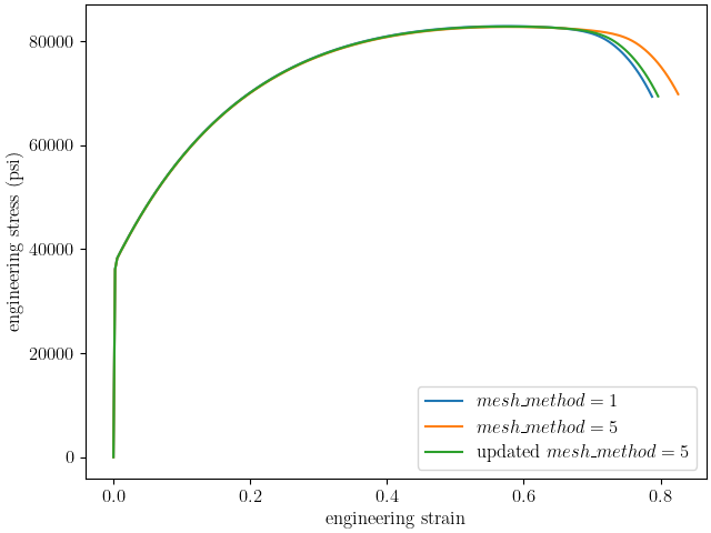
To test that assumption, we will perform a final assessment of the mesh_method = 5 option on the simulation results. For this last simulation, we change the necking_region value for the mesh_method = 5 model in an attempt to obtain better agreement. Since the primary difference in mesh_method = 5 from the other methods is the mesh size reduction at the edge of the necking region, we increase the size of the necking region to see if the results improve.

mesh_method_5.add_constants(necking_region=0.80)
if is_sandia_cluster():
    mesh_method_5.set_number_of_cores(num_cores*2)

We then run just this final model and compare the engineering stress-strain curve to the previous mesh_method = 5 model results and the mesh_method = 1 model results.

updated_mesh_method_5_results = mesh_method_5.run(data_collection.states["batch_fixed_state"], param_collection)
updated_mesh_method_5_results = updated_mesh_method_5_results.results_data


plt.figure(constrained_layout=True)
plt.plot(mesh_method_1_curves["engineering_strain"], mesh_method_1_curves["engineering_stress"], label="$mesh\_method = 1$")
plt.plot(mesh_method_5_curves["engineering_strain"], mesh_method_5_curves["engineering_stress"], label="$mesh\_method = 5$")
plt.plot(updated_mesh_method_5_results["engineering_strain"], updated_mesh_method_5_results["engineering_stress"], label="updated $mesh\_method = 5$")

plt.xlabel("engineering strain")
plt.ylabel("engineering stress (psi)")
plt.legend()
plt.show()

/gpfs/knkarls/projects/matcal_devel/external_matcal/documentation/matcal_model_v_and_v/plot_round_tension_mesh_method_effects.py:246: SyntaxWarning: invalid escape sequence '\_'
  plt.plot(mesh_method_1_curves["engineering_strain"], mesh_method_1_curves["engineering_stress"], label="$mesh\_method = 1$")
/gpfs/knkarls/projects/matcal_devel/external_matcal/documentation/matcal_model_v_and_v/plot_round_tension_mesh_method_effects.py:247: SyntaxWarning: invalid escape sequence '\_'
  plt.plot(mesh_method_5_curves["engineering_strain"], mesh_method_5_curves["engineering_stress"], label="$mesh\_method = 5$")
/gpfs/knkarls/projects/matcal_devel/external_matcal/documentation/matcal_model_v_and_v/plot_round_tension_mesh_method_effects.py:248: SyntaxWarning: invalid escape sequence '\_'
  plt.plot(updated_mesh_method_5_results["engineering_strain"], updated_mesh_method_5_results["engineering_stress"], label="updated $mesh\_method = 5$")

The engineering stress-strain shows that the location of the necking_region border can delay the necking for this mesh method. By moving this transition higher into the gauge section and away from the necking region, it has less of an overall effect on the necking process. This is most likely due to the lower quality elements at the mesh size transition. This effect may be lessened with a less ductile material, but for this study is not negligible.