Note
Go to the end to download the full example code.
304L stainless steel viscoplastic uncertainty quantification validation
In this example, we will use MatCal’s ParameterStudy
to validate the estimated parameter uncertainty for the calibration.
We do this by generating samples from the fitted covariance from
304L stainless steel viscoplastic calibration uncertainty quantification and
running the calibrated models with these samples. Then the
model results are compared to the data to see how well the sampled parameter
sets allow the models to represent the data uncertainty.
To begin, we reuse the data import, model preparation and objective specification for the tension model and rate models from 304L stainless steel viscoplastic calibration uncertainty quantification.
import numpy as np
import matplotlib.pyplot as plt
from matcal import *

plt.rc('text', usetex=True)
plt.rc('font', family='serif')
plt.rc('font', size=12)
figsize = (4,3)

tension_data = BatchDataImporter("ductile_failure_ASTME8_304L_data/*.dat",
                                    file_type="csv")
tension_data.set_fixed_state_parameters(displacement_rate=2e-4, temperature=530)
tension_data = tension_data.batch
tension_data = scale_data_collection(tension_data, "engineering_stress", 1000)
tension_data.remove_field("time")

down_selected_data = DataCollection("down selected data")
for state in tension_data.keys():
   for index, data in enumerate(tension_data[state]):
      down_selected_data.add(data[(data["engineering_stress"] > 36000) &
                                  (data["engineering_strain"] < 0.75)])

rate_data_collection = matcal_load("rate_data.joblib")

calibrated_params = matcal_load("voce_calibration_results.serialized")

Y_0 = Parameter("Y_0", 20, 60,
                calibrated_params["Y_0"])
A = Parameter("A", 100, 400,
              calibrated_params["A"])
b = Parameter("b", 0, 3,
              calibrated_params["b"])
C = Parameter("C", -3, -0.5, calibrated_params["C"])
X = Parameter("X", 0.50, 1.75, 1.0)
params = ParameterCollection("laplace params", Y_0, A, b, C)

def JC_rate_dependence_model(Y_0, A, b, C, X, ref_strain_rate, rate, **kwargs):
    yield_stresses = np.atleast_1d(Y_0*X*(1+10**C*np.log(rate/ref_strain_rate)))
    yield_stresses[np.atleast_1d(rate) < ref_strain_rate] = Y_0
    return {"yield":yield_stresses}

rate_model = PythonModel(JC_rate_dependence_model)
rate_model.set_name("python_rate_model")

material_name = "304L_viscoplastic"
material_filename = "304L_viscoplastic_voce_hardening.inc"
sierra_material = Material(material_name, material_filename,
                            "j2_plasticity")

geo_params = {"extensometer_length": 0.75,
               "gauge_length": 1.25,
               "gauge_radius": 0.125,
               "grip_radius": 0.25,
               "total_length": 4,
               "fillet_radius": 0.188,
               "taper": 0.0015,
               "necking_region":0.375,
               "element_size": 0.01,
               "mesh_method":3,
               "grip_contact_length":1}

astme8_model = RoundUniaxialTensionModel(sierra_material, **geo_params)
astme8_model.add_boundary_condition_data(tension_data)

from site_matcal.sandia.computing_platforms import is_sandia_cluster, get_sandia_computing_platform
from site_matcal.sandia.tests.utilities import MATCAL_WCID

cores_per_node = 24
if is_sandia_cluster():
    platform = get_sandia_computing_platform()
    cores_per_node = platform.processors_per_node

astme8_model.set_number_of_cores(cores_per_node)
if is_sandia_cluster():
    astme8_model.run_in_queue(MATCAL_WCID, 1)
    astme8_model.continue_when_simulation_fails()
astme8_model.set_allowable_load_drop_factor(0.45)
astme8_model.set_name("ASTME8_tension_model")
astme8_model.add_constants(ref_strain_rate=1e-5)

X_calibrated = calibrated_params.pop("X")
rate_model.add_constants(ref_strain_rate=1e-5, X=X_calibrated)
astme8_model.add_constants(ref_strain_rate=1e-5)

rate_objective = Objective("yield")
astme8_objective = CurveBasedInterpolatedObjective("engineering_strain", "engineering_stress")
With the models, data, and objectives created,
we import the LaplaceStudy results from the previous step.
laplace_covariance = matcal_load("laplace_study_covariance.joblib")
Next, we can sample
the calculated parameter distribution using
sample_multivariate_normal() and evaluate
the parameter uncertainty as desired.
num_samples=40
mean = [calibrated_params["Y_0"], calibrated_params["A"],
         calibrated_params["b"], calibrated_params["C"]]
uncertain_param_sets = sample_multivariate_normal(num_samples,
                                                  mean,
                                                  laplace_covariance,
                                                  12345,
                                                  params.get_item_names())
/gpfs/knkarls/projects/matcal_devel/external_matcal/matcal/core/parameter_studies.py:918: RuntimeWarning: covariance is not symmetric positive-semidefinite.
  samples = rng.multivariate_normal(mean, sigma, nsamples).T
We save the parameter samples to be used or plotted later.
matcal_save("laplace_uq_validation_results.joblib", uncertain_param_sets)
Now we set up a study so we can
visualize the results by pushing the samples back through the models.
We do so using a MatCal ParameterStudy.
param_study = ParameterStudy(Y_0, A, b, C)
param_study.add_evaluation_set(astme8_model, astme8_objective, tension_data)
param_study.add_evaluation_set(rate_model, rate_objective, rate_data_collection)
param_study.set_core_limit(250)
sampling_dir = "UQ_sampling_study"
param_study.set_working_directory(sampling_dir, remove_existing=True)
Next, we add parameter evaluations for each of the samples.
We do so by organizing the data using Python’s
zip function and then loop over the result
to add each parameter set sample to the study.
Note
We add error catching to the addition of each parameter evaluation. There is a chance that parameters could be generated outside of our original bounds and we want the study to complete. If this error is caught, we will see it in the MatCal output and know changes are needed. However, some results will still be output and can be of use.
params_to_evaluate = zip(uncertain_param_sets["Y_0"], uncertain_param_sets["A"],
                         uncertain_param_sets["b"], uncertain_param_sets["C"])

for Y_0, A_eval, b_eval, C_eval in params_to_evaluate:
    try:
      param_study.add_parameter_evaluation(Y_0=Y_0, A=A_eval, b=b_eval, C=C_eval)
      print(f"Running evaluation with Y_0={Y_0}, A={A_eval}, b={b_eval}, and "
          f"C={C_eval}.")

    except ValueError:
       print(f"Skipping evaluation with Y={Y_0}, A={A_eval}, b={b_eval}, and "
            f"C={C_eval}. Parameters out of range.")
Running evaluation with Y_0=40.72441342703886, A=182.4379144883937, b=1.4698690626316924, and C=-1.9661180231567008.
Running evaluation with Y_0=32.393486456122886, A=161.19478113745876, b=2.006511861609928, and C=-1.3498419855317558.
Running evaluation with Y_0=28.452810086690572, A=154.53948380147227, b=2.0374150528005344, and C=-0.9408999658855374.
Running evaluation with Y_0=38.010725023703465, A=171.72381021836316, b=1.6895835276696582, and C=-1.7298186757585254.
Running evaluation with Y_0=28.766099706537293, A=147.27714013159462, b=2.249412459359706, and C=-0.9725980021826655.
Running evaluation with Y_0=29.350567334533224, A=138.18231240696633, b=2.3183375888108753, and C=-1.041766366545879.
Running evaluation with Y_0=35.27398131988298, A=162.0794566342244, b=1.9351683687561434, and C=-1.5485637758316813.
Running evaluation with Y_0=34.67763708386793, A=130.46006188864052, b=2.464860447431711, and C=-1.2551337273650789.
Running evaluation with Y_0=33.89531959164911, A=175.81704154012397, b=1.7174942325839184, and C=-1.5173311381157752.
Running evaluation with Y_0=30.194844392177533, A=147.6451229375477, b=2.267451064349489, and C=-1.1573626767841783.
Running evaluation with Y_0=32.63388591315658, A=154.60915613447523, b=2.000587273735786, and C=-1.2620956404737014.
Running evaluation with Y_0=31.55514090058545, A=161.18874089889496, b=1.975060235421476, and C=-1.2261280144861153.
Running evaluation with Y_0=33.80573861940592, A=158.6439707400068, b=1.9549016564098698, and C=-1.3706013757772066.
Running evaluation with Y_0=33.48844008845267, A=150.79508763959453, b=2.0682396461474486, and C=-1.3383337771223938.
Running evaluation with Y_0=29.39802042512996, A=155.39857540469103, b=2.034913879600619, and C=-1.141190710352086.
Running evaluation with Y_0=35.080306871627954, A=160.64921258131145, b=1.9315560569894779, and C=-1.4921334937991544.
Running evaluation with Y_0=36.637880765569946, A=186.8101218586871, b=1.3534286190619456, and C=-1.714389913372552.
Running evaluation with Y_0=28.86420228823914, A=149.58943259128296, b=2.1997042497147175, and C=-1.1162228528410867.
Running evaluation with Y_0=34.986977166358336, A=159.34441780985583, b=1.975436533340711, and C=-1.5110756691801719.
Running evaluation with Y_0=28.4505275045769, A=133.29544710198115, b=2.5402686618897072, and C=-0.9631604893152708.
Running evaluation with Y_0=32.90690664580745, A=163.60271329192219, b=1.9773242694403805, and C=-1.4024767994618468.
Running evaluation with Y_0=35.46877875187567, A=169.0022277303849, b=1.8299804768263006, and C=-1.5433985875507392.
Running evaluation with Y_0=33.85014930972343, A=147.06577777988235, b=2.194593519115062, and C=-1.3292175404196238.
Running evaluation with Y_0=33.53257795557018, A=144.7164837386597, b=2.2111322204432784, and C=-1.2996204964524651.
Running evaluation with Y_0=33.19386471967011, A=165.83994480464247, b=1.8875270060013802, and C=-1.4156286373270253.
Running evaluation with Y_0=30.096100054944113, A=164.45297769614643, b=1.9368154564613362, and C=-1.1731027411795758.
Running evaluation with Y_0=30.500180089918693, A=164.89698140606384, b=1.9152141140448151, and C=-1.2068830898894893.
Running evaluation with Y_0=32.29796086482621, A=156.53914128321043, b=1.9979403316304873, and C=-1.1716628948496.
Running evaluation with Y_0=35.91492059998702, A=160.95928948111384, b=1.9013168782329948, and C=-1.4953225008433946.
Running evaluation with Y_0=31.461520572465364, A=135.60266014588237, b=2.3979782443614477, and C=-1.155426544539657.
Running evaluation with Y_0=36.10480404265594, A=172.9460321355645, b=1.6348363141299118, and C=-1.5538043446418954.
Running evaluation with Y_0=34.24280847540498, A=158.70316244278564, b=1.9713866266222762, and C=-1.4029721979682204.
Running evaluation with Y_0=32.66430447288298, A=178.79600037455202, b=1.5941086037490335, and C=-1.474231700574034.
Running evaluation with Y_0=28.819901430442126, A=133.34271030751583, b=2.462315108734435, and C=-1.023622947668414.
Running evaluation with Y_0=31.629861183239814, A=155.30728898079195, b=2.0301635592986917, and C=-1.1823384892781248.
Running evaluation with Y_0=36.9618161227402, A=172.18786311148634, b=1.7677307599738525, and C=-1.7658475756813192.
Running evaluation with Y_0=31.99216740163429, A=138.99780057322496, b=2.3416666175073373, and C=-1.182426967568504.
Running evaluation with Y_0=34.891225833580656, A=183.4007024432691, b=1.532075399508311, and C=-1.521329077103156.
Running evaluation with Y_0=41.46816614902843, A=194.89417599665467, b=1.20389579843005, and C=-1.985068245620005.
Running evaluation with Y_0=35.1471425513697, A=174.08117376999581, b=1.6352887894457413, and C=-1.5802683407957228.
Next, we launch the study and plot the results. Once again, we use plotting functions from the previous examples to simplify the plotting processes.
param_study_results = param_study.launch()
astme_results = param_study_results.simulation_history[astme8_model.name]
rate_results = param_study_results.simulation_history[rate_model.name]
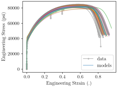
def compare_data_and_model(data, model_responses, indep_var, dep_var,
plt_func=plt.plot, fig_label=""):
fig = plt.figure(fig_label, constrained_layout=True, figsize=figsize)
data.plot(indep_var, dep_var, plot_function=plt_func, ms=3, labels="data",
figure=fig, marker='o', linestyle='-', color="#bdbdbd", show=False)
model_responses.plot(indep_var, dep_var, plot_function=plt_func,labels="models",
figure=fig, linestyle='-', alpha=0.5)
plt.xlabel("Engineering Strain (.)")
plt.ylabel("Engineering Stress (psi)")
compare_data_and_model(tension_data, astme_results,
"engineering_strain", "engineering_stress",
fig_label="tension model")
def make_single_plot(data_collection, state, cur_idx, label,
color, marker, **kwargs):
data = data_collection[state][cur_idx]
plt.semilogx(state["rate"], data["yield"][0],
marker=marker, label=label, color=color,
**kwargs)
def plot_dc_by_state(data_collection, label=None, color=None,
marker='o', best_index=None, only_label_first=False, **kwargs):
for state in data_collection:
if best_index is None:
for idx, data in enumerate(data_collection[state]):
make_single_plot(data_collection, state, idx, label,
color, marker, **kwargs)
if ((color is not None and label is not None) or
only_label_first):
label = None
else:
make_single_plot(data_collection, state, best_index, label,
color, marker, **kwargs)
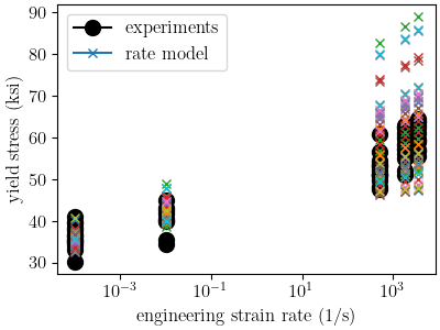
plt.xlabel("engineering strain rate (1/s)")
plt.ylabel("yield stress (ksi)")
plt.figure(constrained_layout=True, figsize=figsize)
plot_dc_by_state(rate_data_collection, label='experiments',
color="k", markersize=10)
plot_dc_by_state(rate_results, label='rate model', marker='x',
only_label_first=True)
plt.legend()
/gpfs/knkarls/projects/matcal_devel/external_matcal/matcal/core/data.py:588: UserWarning: Ignoring specified arguments in this call because figure with num: 1 already exists
  plt.figure(figure.number, constrained_layout=True)

<matplotlib.legend.Legend object at 0x1554bd6212e0>
These figure show the model results from the 40 samples. For the tension model, the results appear to be good estimate of parameter uncertainty. The simulations encapsulate all data, without exhibiting too much variability. While the python rate dependence model results do not completely encapsulates all data, the results seem to be an adequate measure of overall uncertainty.
Total running time of the script: (12 minutes 32.609 seconds)