Model Identifiability Issue Example

In this example the underlying data model is linear, and the fitted model is over-parameterized i.e., is too complex for the data. There are too many parameters to fit the data uniquely, and this is not due to the number of data points. It is due to the form of the model (it is bilinear) vs. the trend in the data (it is just linear). Since the error contours are not closed, there is no unique best fit as the calibration is formulated. The data should indicate that H = E, but nothing informs what Y should be. Although simplistic, this case is emblematic of the calibration of some material models. More complex cases with nonlinearities can exhibit multiple wells with multiple optima. There are ways of combating this such as L1 regularization of the parameters that add a small cost to calibrating non-zero parameters.

from matcal import *
import numpy as np

We create a python function to be used as a MatCal PythonModel for this calibration. The python model uses Numpy in the function and requires that Numpy be imported within the function. As stated above, the data will be fitted to a model with a bilinear response similar to an elastic-plastic model. The initial slope (E) is assumed to be known. The parameter “Y” determines where the model changes to the second linear trend and the parameters “H” determines the second slope.

def bilinear_model(Y, H, npoints=100):
  import numpy as np
  max_strain = 1.0
  strain = np.linspace(0,max_strain,npoints)
  E = 1.5
  eY = Y/E
  stress = np.where(strain < eY, E*strain, Y + H*(strain-eY))
  response = {'strain':strain, 'stress': stress}
  return response

With the function for the model defined above, we create the parameters for our MatCal calibration study and the MatCal PythonModel from the function.

Y = Parameter('Y',0.0,1.0, 0.5)
H = Parameter('H',0.0,2.0, 0.5)
parameters = ParameterCollection('parameters', Y, H)
model = PythonModel(bilinear_model)

A simple gradient-based calibration with a mean squared error objective is enough to illustrate the point. We create the data, create the calibration based on the model parameters, and define an objective for fitting the model response to the data.

nexp_points=30
def generate_data(stddev):
    data = bilinear_model(Y=0.5, H=1.5, npoints=nexp_points)
    from numpy.random import default_rng
    _rng = default_rng(seed=12345)
    data['stress'] += stddev*_rng.standard_normal(len(data["stress"]))
    data = convert_dictionary_to_data(data)
    return data
data = generate_data(stddev=0)
calibration = GradientCalibrationStudy(parameters)
objective = CurveBasedInterpolatedObjective('strain','stress')
calibration.add_evaluation_set(model, objective, data)

We can then run the calibration and select the optimal parameters and the best fit.

results = calibration.launch()
best_parameters = results.best.to_dict()
best_response = results.best_simulation_data(model, 'matcal_default_state')

First, compare the response curves. We plot the calibrated model with lines and the data with points. We can see that an acceptable fit has been found.

import matplotlib.pyplot as plt
plt.figure()
plt.plot(best_response['strain'],best_response['stress'],'b',label="fit")
plt.scatter(data['strain'],data['stress'],2,'r',label="data")
plt.xlabel("STRAIN")
plt.ylabel("STRESS")

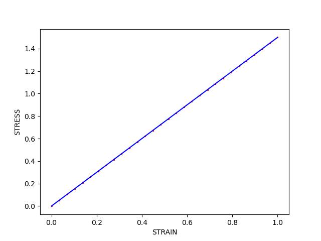
Text(42.597222222222214, 0.5, 'STRESS')

However, we know that the parameter Y should have no effect. Next, examine how the error changes in the vicinity of the best fit. This a helper function to evaluate the error on a grid of parameter values for plotting. MatCal’s ParameterStudy can also do this.

def sample_error(model, data, ranges = {"Y":[0.0,1.0],"H":[0.0,2.0]} ):
  Ys, Hs = np.mgrid[ ranges["Y"][0]:ranges["Y"][1]:100j, ranges["H"][0]:ranges["H"][1]:100j]
  Zs = np.empty_like(Ys)
  for i in range(Ys.shape[0]):
    for j in range(Ys.shape[1]):
      parameters = {"Y":Ys[i,j],"H":Hs[i,j]}
      response = model(**parameters, npoints=nexp_points)
      residual = response['stress']-data['stress']
      error = np.sum(residual**2)
      Zs[i,j] = error
  return Ys,Hs,Zs

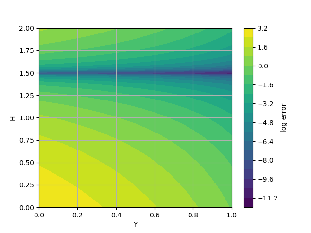
The contour plot depicts the change in error.

Ys,Hs,Zs = sample_error(bilinear_model,data)
plt.figure()
plt.contourf(Ys,Hs,np.log(Zs),20)
plt.grid(True)
plt.xlabel("Y")
plt.ylabel("H")
plt.colorbar(label="log error")

<matplotlib.colorbar.Colorbar object at 0x155517c05ee0>

Note that there are no closed contours, and so, no optima. Any Y value with the correct H value gives equivalent errors. The problem is not “well-posed” as we constructed it. Removing or setting the “Y” parameter is the easiest fix; however, with more complex models this issue and its remedy might not be as apparent.

If we run the calibration again with a new initial point, we can again get a calibrated result.

parameters.update_parameters(Y=0.1, H=0.3)
calibration = GradientCalibrationStudy(parameters)
objective = CurveBasedInterpolatedObjective('strain','stress')
calibration.add_evaluation_set(model, objective, data)

After we run the calibration, we inspect the new results and see that a different value of Y has been provided.

results = calibration.launch()
best_parameters_different_start = results.best.to_dict()
print("Initial best:", best_parameters)
print("Updated best:", best_parameters_different_start)

Initial best: OrderedDict({'Y': 0.5, 'H': 1.5})
Updated best: OrderedDict({'Y': 0.1, 'H': 1.5})

One way of determining the identifiability of the parameters is to determine the curvature of the objective around the found minima. If the curvature is low or zero, the parameter cannot be well identified at least with the current objective(s). The objective function curvature can be obtained using our ClassicLaplaceStudy which calculates the hessian of objective function around a point in the objective space.

Note

The hessian is approximated using finite differencing which can be very expensive for models will large numbers of parameters.

Warning

Our finite differencing currently does not account for parameter bounds. Errors may result, so update the center such that parameter values are not on the bounds.

study = ClassicLaplaceStudy(Y, H)
best_H = best_parameters_different_start["H"]
best_Y = best_parameters_different_start["Y"]
study.set_parameter_center(H=best_H, Y=best_Y-1e-8)
study.set_step_size(1e-8)
study.add_evaluation_set(model, objective, data)
study.run_in_serial()
results = study.launch()

After running the study, we inspect the hessian and see that the hessian with respect to Y is essentially zero at this point.

print(results.parameter_order)
print(results.hessian)

['Y', 'H']
[[1.04372529e-17 5.76634997e-10]
 [5.76634997e-10 2.45934010e-01]]

However, for real data with model form error and noise it might not be so apparent. If we re-generate data with noise and re-run the ClassicLaplaceStudy, we can see the hessian of the objective with respect to Y is now non-zero, but small. We have to find the new minimum before evaluating at the hessian.

data = generate_data(0.05)
parameters.update_parameters(Y=0.25, H=0.25)
calibration = GradientCalibrationStudy(parameters)
objective = CurveBasedInterpolatedObjective('strain','stress')
calibration.add_evaluation_set(model, objective, data)
results = calibration.launch()
best_parameters = results.best.to_dict()
best_response = results.best_simulation_data(model, 'matcal_default_state')

plt.figure()
plt.plot(best_response["strain"],best_response["stress"],'b',label="fit")
plt.scatter(data["strain"],data["stress"],2,'r',label="data")
plt.xlabel("STRAIN")
plt.ylabel("STRESS")
print(best_parameters)

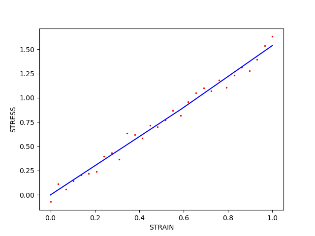
OrderedDict({'Y': 0.88570574171, 'H': 1.5953968607})

With the new optimum found, we run the ClassicLaplaceStudy and inspect the new results.

study = ClassicLaplaceStudy(Y, H)
best_H = best_parameters["H"]
best_Y = best_parameters["Y"]
study.set_parameter_center(H=best_H, Y=best_Y+3e-8)
study.set_step_size(1e-8)
study.add_evaluation_set(model, objective, data)
study.run_in_serial()
results = study.launch()
print(results.parameter_order)
print(results.hessian)
print(np.linalg.eig(results.hessian))
plt.show()

['Y', 'H']
[[ 0.00195312 -0.00439453]
 [-0.00439453  0.02246094]]
EigResult(eigenvalues=array([0.00105111, 0.02336295]), eigenvectors=array([[-0.97957772,  0.20106587],
       [-0.20106587, -0.97957772]]))

We can see that hessian of the objective with respect to Y is no longer zero, but it is lower than the hessian with respect to H. This indicates Y may not be well identified by the objective. However, it is not immediately obvious that it cannot be identified. The hessian now has non-zero eigen values and is positive definite, indicating the model might have a local minima at the calibrated point. Noise can create a minimum or local minima in cases such as the one shown here.