Latin Hypercube Sampling to Obtain Local Material Sensitivities

In this section, we will cover how to run a Latin Hypercube Sampling study using a model from an external physics modeling software. MatCal is written to be modular, so any tools taught here can be mixed and matched with tools presented in other examples. This example builds on the work done in the previous section, Calibration of Two Different Material Conductivities. The points discussed in this example will be used to elucidate the differences in setup between a calibration study and a sensitivity study.

If you want more details about particular types of studies please see MatCal Studies.

After performing our calibration in the previous example, we want to know how important our conductivities are to our prediction. To do this, we want to get a measure of our solution’s sensitivity to our parameters. Fortunately for us, we have done much of the hard work already for the calibration, and we can just change a few lines in our MatCal script to perform a Latin Hypercube Sampling study and get Pearson correlation values. Pearson correlations tell us how correlated our parameters are with our quantities of interest. For this study, we can begin by adapting our MatCal input from the previous example.

from matcal import *
import numpy as np

cond_1 = Parameter("K_foam", .1 , .2, distribution="uniform_uncertain")
cond_2 = Parameter("K_steel", 30, 60, distribution="uniform_uncertain")

We start our MatCal input the same way we did with the calibration, by importing MatCal and defining our parameters. However, we are only attempting to asses how sensitive our model is to the parameters over the range of interest. As a result, data do not need to be supplied. We just need to define what fields we are interested in from the model results and at what independent values and states we want these data. To that end, we create the state of interest and independent values of interest below.

low_flux_state = State("LowFlux", exp_flux=1e3)
import numpy as np
independent_field_values = np.linspace(0,20,11)

The objective for this study will be a SimulationResultsSynchronizer. Since we do not need to compare to data for this study, this is will synchronize simulation results to common independent field values that are user specified for comparison. For MatCal, the synchronizer behaves like an objective and is comparing the simulation results to a vector of zeros for each dependent field. As a result, there is no data conditioning, normalization or weighting applied to the simulation results.

objective = SimulationResultsSynchronizer("time", independent_field_values,
                                          "T_middle", "T_bottom")

Next, we set up our model and objective just as we did in the calibration example.

user_file = "two_material_square.i"
geo_file = "two_material_square.g"
sim_results_file = "two_material_results.csv"
model = UserDefinedSierraModel('aria', user_file, geo_file)
model.set_results_filename(sim_results_file)

The last difference between the calibration study and this sensitivity study is our choice of study. In this example we are using a LhsSensitivityStudy. We initialize it and add our evaluation set to it as is common MatCal study procedure. In this study we are just looking at one state. However, multiple states can be run if desired through the states keyword argument.

sens = LhsSensitivityStudy(cond_1, cond_2)
sens.add_evaluation_set(model, objective, states=low_flux_state)
sens.set_core_limit(48)

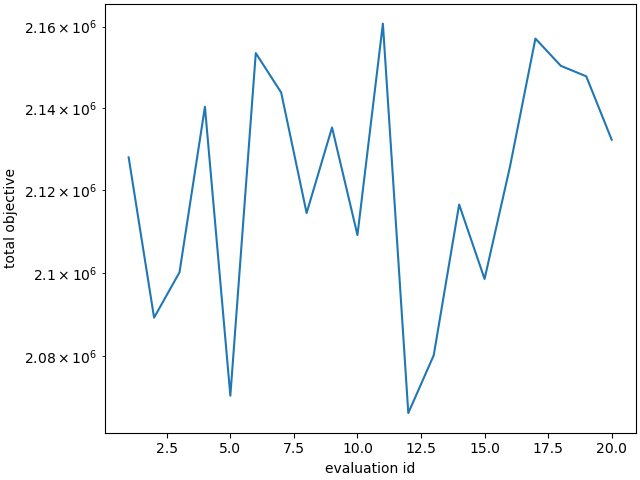
The last input needed is how many samples to take in the LHS study. The study needs a certain number of samples to produce a converged solution; however, that number is problem dependent. We will likely have to run our study a few times to confirm we have a converged solution. A decent starting guess is ten times the number of parameters you are studying. As a result, we set the number of samples to 20.

sens.set_number_of_samples(20)

Now all that is left to do is to launch the study and wait for our results.

results = sens.launch()
print("Pearson coefficients\n", results.pearson)
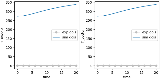
make_standard_plots('time')

• 
• 
• 

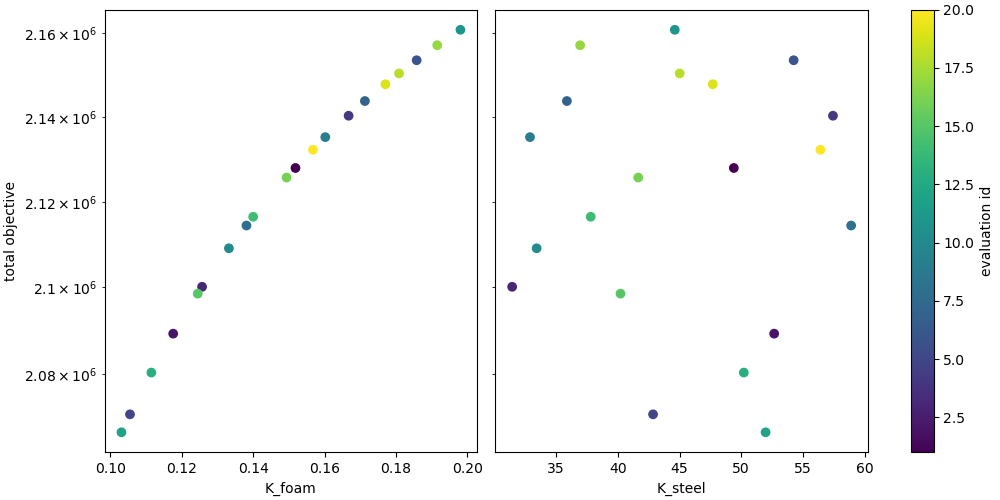
Pearson coefficients
 K_foam: [     nan 0.999528 0.995936 0.992279 0.989029 0.986511 0.984599 0.983165
 0.982134 0.981413 0.980732      nan 0.999548 0.995984 0.992346 0.989114
 0.986616 0.984725 0.983314 0.982309 0.981615 0.980965]
K_steel: [       nan -0.200358  -0.133949  -0.132451  -0.137034  -0.143376
 -0.150147  -0.157224  -0.164632  -0.172227  -0.180501         nan
  0.0855372 -0.0546177 -0.0747372 -0.084218  -0.0896342 -0.0929785
 -0.0950772 -0.0962743 -0.0968421 -0.0972399]

We now repeat the study, but request Sobol Indices to be output.

sens = LhsSensitivityStudy(cond_1, cond_2)
sens.set_random_seed(1702)
sens.add_evaluation_set(model, objective, states=low_flux_state)
sens.set_core_limit(48)
sens.set_number_of_samples(20)
sens.make_sobol_index_study()
results = sens.launch()

Notice that much more examples are now run. For a study producing Sobol indices, Dakota will run samples where is the number of requested samples and is the number of study parameters in the study. As a result, for this study a total of 80 samples are run.

print("Sobol indices:\n", results.sobol)

Sobol indices:
 K_foam: [[0.94134083 0.94356568]
 [0.94718918 0.9531443 ]
 [0.95128463 0.95956404]
 [0.95447247 0.96447351]
 [0.95673064 0.96796421]
 [0.95830848 0.97044516]
 [0.95937994 0.97218598]
 [0.9600381  0.97332616]
 [0.96038377 0.97400478]
 [0.96064815 0.97457472]
 [0.9447975  0.94527186]
 [0.94932542 0.9544026 ]
 [0.95308511 0.96077249]
 [0.95620779 0.96577022]
 [0.95852461 0.96941623]
 [0.96022202 0.97209166]
 [0.96145681 0.97405761]
 [0.96231566 0.97545085]
 [0.96289199 0.97640461]
 [0.96342324 0.97729313]]
K_steel: [[-1.19619581e-03  2.85182485e-05]
 [-9.18943150e-04  1.57997927e-05]
 [-9.17387135e-04  1.58243175e-05]
 [-1.02191575e-03  2.01410339e-05]
 [-1.19221883e-03  2.80931532e-05]
 [-1.40371495e-03  3.97827196e-05]
 [-1.65161213e-03  5.60700807e-05]
 [-1.93385708e-03  7.81054766e-05]
 [-2.24235215e-03  1.06585123e-04]
 [-2.58797334e-03  1.44413426e-04]
 [ 1.04036755e-03  2.18186638e-05]
 [ 8.53195655e-04  1.40247417e-05]
 [ 8.33276291e-04  1.30954406e-05]
 [ 8.67101453e-04  1.39710167e-05]
 [ 9.22249565e-04  1.56327447e-05]
 [ 9.83891608e-04  1.76275232e-05]
 [ 1.04787534e-03  1.97898463e-05]
 [ 1.11055835e-03  2.19912538e-05]
 [ 1.16588918e-03  2.39837019e-05]
 [ 1.22336584e-03  2.61418944e-05]]

As can bee seen above, there are some unexpected results. The method provides the sensitivity indices for main effects and the total effects for each parameter, respectively. The main effects are representative of the contribution of each study parameter the variance in the model response. While the total effects represent the contribution of each parameter in combination with all the other parameters to the variance in the model response.

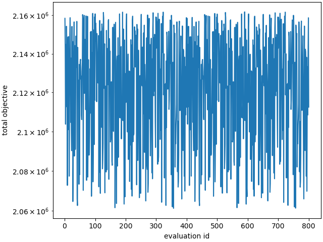
For both cases the result should be positive. However, in these results the K_steel parameter has some negative values. This is most likely due to the sampling size being too small and the fact that the index values are small. As a result, numerical errors cause the values to become negative. To investigate this issue we re-run the study with more samples. This time we choose a sample size of 200, which will run a total of 800 models. Dakota’s documentation recommends hundreds to thousands of samples for a sampling study producing Sobol indices.

sens = LhsSensitivityStudy(cond_1, cond_2)
sens.add_evaluation_set(model, objective, states=low_flux_state)
sens.set_core_limit(48)
sens.set_random_seed(1702)
sens.set_number_of_samples(200)
sens.make_sobol_index_study()
results = sens.launch()
print("Updated Sobol indices:\n", results.sobol)

Updated Sobol indices:
 K_foam: [[1.01729177 1.01815039]
 [1.01632713 1.01745161]
 [1.01581985 1.01707549]
 [1.01540227 1.01675873]
 [1.01502117 1.01646154]
 [1.01467344 1.01618765]
 [1.01435519 1.01593714]
 [1.01406974 1.01571509]
 [1.01382922 1.01553424]
 [1.01357718 1.01534713]
 [1.01754963 1.01863023]
 [1.01652001 1.01763749]
 [1.01602055 1.01719073]
 [1.01563524 1.01685226]
 [1.01530049 1.01655276]
 [1.01500866 1.01628655]
 [1.01475627 1.01605209]
 [1.01454748 1.01585433]
 [1.01439286 1.0157053 ]
 [1.01424405 1.01556047]]
K_steel: [[-5.93538202e-05  2.43937396e-05]
 [-2.86560337e-05  1.47345748e-05]
 [-2.70083895e-05  1.51291295e-05]
 [-3.06401276e-05  1.94139954e-05]
 [-3.40218824e-05  2.71778318e-05]
 [-3.58288668e-05  3.85878687e-05]
 [-3.47026406e-05  5.45095512e-05]
 [-2.94062033e-05  7.60959479e-05]
 [-1.88814599e-05  1.04054920e-04]
 [-1.64752497e-06  1.41266760e-04]
 [ 1.08084036e-04  1.76967938e-05]
 [ 6.60797538e-05  1.24762318e-05]
 [ 5.75503936e-05  1.21701080e-05]
 [ 5.73054632e-05  1.33173683e-05]
 [ 5.98862461e-05  1.51329738e-05]
 [ 6.37180626e-05  1.72411691e-05]
 [ 6.79094183e-05  1.95078353e-05]
 [ 7.20202832e-05  2.18105940e-05]
 [ 7.53833850e-05  2.39035493e-05]
 [ 7.88162506e-05  2.61772375e-05]]

In these results, we see that all of the indices have changed significantly. This indicates that the Sobol indices are likely not converged. For a real problem, users should continue running studies with increasing samples until the indices converge. Also, regarding the negative values from the 20 sample study, some values are still negative. This is likely due to them being near zero and within expected numerical errors with the number of samples. If we were to do a proper sample size convergence study, these would continue decreasing in magnitude but may never turn all positive. Although potentially not converged, we can plot the current results and make conclusions about the influence of the parameters on our QoIs.

make_standard_plots('time')

• 
• 
• 

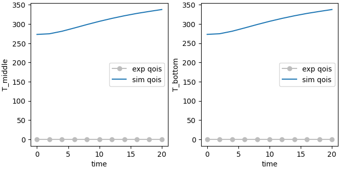
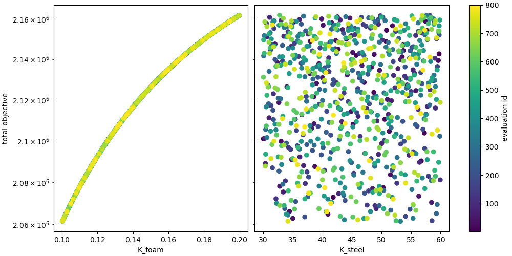
In these results, we see that across all time the conductivity of the foam has a strong correlation with both of our temperature values of interest, while the conductivity of steel has very little. This indicates that this experimental series is likely a good approach for determining a foam conductivity, however, is less useful in determining the steel conductivity. It would be useful to find another set of data to help us study the steel.