Load Displacement Calibration Verification - First Attempt

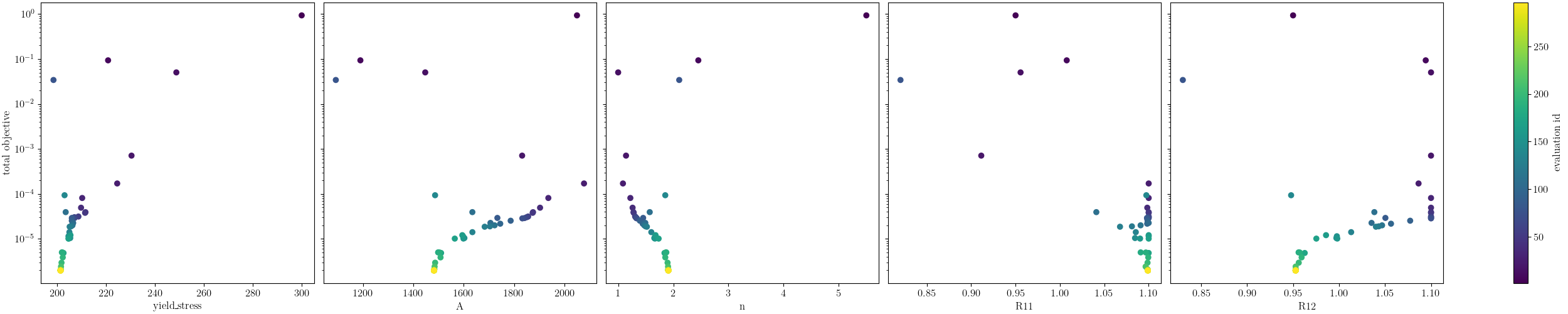
In this example, we attempt to calibrate the five parameters of our verification problem using only the load-displacement curve. Since the Objective Sensitivity Study shows that the objective is at a minimum it should be possible. However, since the model is fairly expensive we attempt to do so using a gradient method. Specifically, we use the GradientCalibrationStudy using Dakota’s nl2sol method implementation. 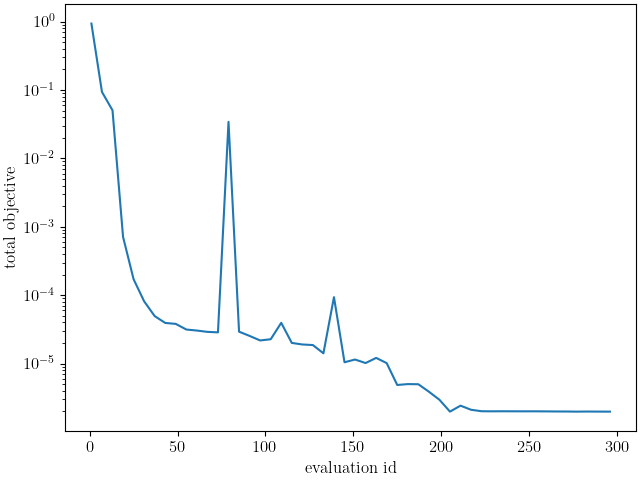As we will see, the objective is difficult to calibrate due to the observed discontinuities and likely local minima throughout the parameter space. As a result, the method fails with little progress.

To begin we import the MatCal tools necessary for this study and import the data that will be used for the calibration.

from matcal import *
import numpy as np
import matplotlib.pyplot as plt

plt.rc('text', usetex=True)
plt.rc('font', family='serif')
plt.rcParams.update({'font.size': 12})

Next, we import the data we wish to use in the study. For this study, we import the Exodus data from the 0_degree synthetic data set.

synthetic_data = FieldSeriesData("../../../docs_support_files/synthetic_surf_results_0_degree.e")

You are using exodus.py v 1.21.6 (seacas-py3), a python wrapper of some of the exodus library.

Copyright (c) 2013-2023 National Technology &
Engineering Solutions of Sandia, LLC (NTESS).  Under the terms of
Contract DE-NA0003525 with NTESS, the U.S. Government retains certain
rights in this software.

Opening exodus file: ../../../docs_support_files/synthetic_surf_results_0_degree.e
Opening exodus file: ../../../docs_support_files/synthetic_surf_results_0_degree.e
Closing exodus file: ../../../docs_support_files/synthetic_surf_results_0_degree.e
Closing exodus file: ../../../docs_support_files/synthetic_surf_results_0_degree.e

After importing the data, we select the data we want for our study. For the load-displacement curve objective, we want all time steps up to 92.5% of peak load past peak load. These data are selected for the synthetic_data object below using NumPy array slicing and tools. We do this because we only run the simulation until its load has dropped to 92.5% of peak load after peak load. As stated previously, this is done for model robustness and to reduce simulation time. For certain parameters in the available parameter space, peak load will occur early in the displacement space and the model will not be able to run to the expected displacement. With adaptive time stepping, the model will run for an extended period without significant progress and use up valuable resources. We force the model to exit to avoid this. The discontinuity this introduces is unavoidable as the model cannot run successfully for any set of input parameters.

peak_load_arg = np.argmax(synthetic_data["load"])

desired_arg = np.argmin(np.abs(synthetic_data["load"]\
                               [peak_load_arg:]-np.max(synthetic_data["load"])*0.925))
synthetic_data = synthetic_data[:desired_arg+1+peak_load_arg]

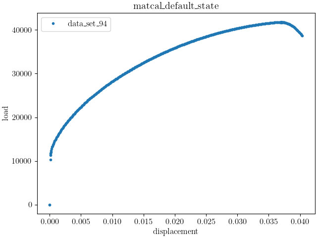
With the data imported and selected, we plot the data to verify our data manipulation.

dc = DataCollection("data", synthetic_data)
dc.plot("displacement", "load")

After importing and preparing the data, we create the model that will be used to simulate the characterization test. We will use a UserDefinedSierraModel for this example. We setup the model input to require an external SierraSM material model input file. We create it next using python string and file tools.

mat_file_string = """begin material test_material
  density = 1
  begin parameters for model hill_plasticity
    youngs modulus  = {elastic_modulus*1e9}
    poissons ratio  = {poissons}
    yield_stress    = {yield_stress*1e6}

    hardening model = voce
    hardening modulus = {A*1e6}
    exponential coefficient = {n}

    coordinate system = rectangular_coordinate_system

    R11 = {R11}
    R22 = {R22}
    R33 = {R33}
    R12 = {R12}
    R23 = {R23}
    R31 = {R31}
  end
end
"""

with open("modular_plasticity.inc", 'w') as fn:
    fn.write(mat_file_string)

With the material file created, the model can be instantiated. We provide the UserDefinedSierraModel with the correct user supplied input deck and mesh. For this model, we use adagio as the simulation solid mechanics code. Next, we use the appropriate model methods to setup the model for the study. Most importantly we pass the correct model constants to it and provide the model with the correct results model output information. The model constants passed to the model are the uncalibrated parameters described in Full-field Verification Problem Material Model.

model = UserDefinedSierraModel("adagio", "synthetic_data_files/test_model_input_reduced_output.i",
                               "synthetic_data_files/test_mesh.g", "modular_plasticity.inc")
model.set_name("test_model")
model.add_constants(elastic_modulus=200, poissons=0.27, R22=1.0, R33=0.9, R23=1.0, R31=1.0)
model.read_full_field_data("surf_results.e")
from site_matcal.sandia.computing_platforms import is_sandia_cluster, get_sandia_computing_platform
from site_matcal.sandia.tests.utilities import MATCAL_WCID
num_cores=96
if is_sandia_cluster():
    platform = get_sandia_computing_platform()
    num_cores = platform.get_processors_per_node()
    model.run_in_queue(MATCAL_WCID, 0.5)
    model.continue_when_simulation_fails()
model.set_number_of_cores(num_cores)

We now create the objective that will be used for the calibration. The independent variable is the “displacement” and the calibration residual is determined from the “load” result. The right=0 informs the objective to provide a zero value for loads if it is forced to extrapolate. This occurs when the simulation plastically localizes and exits before its displacement reaches the maximum displacement of the synthetic data. It contributes to the observed objective discontinuity.

load_objective = CurveBasedInterpolatedObjective("displacement", "load", right=0)
load_objective.set_name("load_objective")

We then create the material model input parameters for the study. We provide realistic bounds that one may expect for an austenitic stainless steel based on our experience with the material. This results in an initial point far from the true values used for the synthetic data generation and is a stressing test for a local gradient based method.

Y = Parameter("yield_stress", 100, 500.0)
A = Parameter("A", 100, 4000)
n = Parameter("n", 1, 10)
R11 = Parameter("R11", 0.8, 1.1)
R12 = Parameter("R12", 0.8, 1.1)

param_collection = ParameterCollection("Hill48 in-plane", Y, A, n, R11, R12)

Finally, we create the calibration study and pass the parameters relevant to the study during its initialization. We then set the total cores it can use locally and pass the data, model and objective to it as an evaluation set.

study = GradientCalibrationStudy(param_collection)
study.set_results_storage_options(results_save_frequency=len(param_collection)+1)
study.set_core_limit(100)
study.add_evaluation_set(model, load_objective, synthetic_data)
study.set_working_directory("load_disp_cal_initial", remove_existing=True)
study.set_step_size(1e-4)
study.do_not_save_evaluation_cache()

Next we launch the study save the results.

results = study.launch()

When the study completes, we extract the calibrated parameters and evaluate the error.

calibrated_params = results.best.to_dict()
print(calibrated_params)

goal_results = {"yield_stress":200,
                "A":1500,
                "n":2,
                "R11":0.95,
                "R12":0.85}

def pe(result, goal):
    return (result-goal)/goal*100

for param in goal_results.keys():
    print(f"Parameter {param} error: {pe(calibrated_params[param], goal_results[param])}")

OrderedDict({'yield_stress': 201.38720848, 'A': 1481.7593516, 'n': 1.9106662899, 'R11': 1.099055052, 'R12': 0.95279046881})
Parameter yield_stress error: 0.6936042399999991
Parameter A error: -1.2160432266666703
Parameter n error: -4.466685505000001
Parameter R11 error: 15.690005473684213
Parameter R12 error: 12.092996330588234

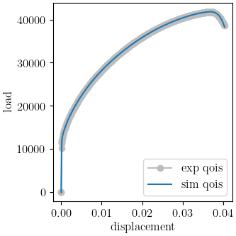
These error’s are much higher than desired for a successful calibration. This is expected as the problem was designed to have non-unique solutions when calibrating only to the load-displacement curves. Using MatCal’s standard plot, we can see that the load-displacement curve matches quite well. In the follow-on, examples we will show how adding full-field data improves results and how the different full-field methods perform.

import os
init_dir = os.getcwd()
os.chdir("load_disp_cal_initial")
make_standard_plots("displacement")
os.chdir(init_dir)

# sphinx_gallery_thumbnail_number = 2

• 
• 
•