Full-field Interpolation Calibration Verification - Success!

This example is a repeat of the Full-field Interpolation Calibration Verification with a simplification of the full-field interpolating objective.

There are two differences in this calibration that allows it to be successful where the referenced example above fails.

1. We choose to only compare data at peak load. This seems to improve the objective landscape near the true global minimum. When comparing the full-field data at multiple points in the load displacement curve, some fields may improve while others get worse. This may make the search methods unable to choose an appropriate search direction. By choosing the single step at peak load, we avoid this issue. We choose the step at peak load because it contains data where the part is highly-deformed which is relevant to the plasticity model we are calibrating

2. We choose an initial point that is only 4% away from the known solution. For this calibration we must be near the known solution for the calibration to converge using gradient methods. In real calibrations, the true solution is not known, so a non-gradient method may be needed as a first step to identify regions where the objective is lowest. Gradient calibrations can then be started from these locations to drive down to the local minima.

All other inputs remain the same. As a result, the commentary is mostly removed for this example except for some discussion on the results at the end.

from matcal import *
import numpy as np

synthetic_data = FieldSeriesData("../../../docs_support_files/synthetic_surf_results_0_degree.e")
synthetic_data.rename_field("U", "displacement_x")
synthetic_data.rename_field("V", "displacement_y")
synthetic_data.rename_field("W", "displacement_z")

peak_load_arg = np.argmax(synthetic_data["load"])
last_desired_arg = np.argmin(np.abs(synthetic_data["load"][peak_load_arg:]
                                    -np.max(synthetic_data["load"])*0.925))
synthetic_data = synthetic_data[:last_desired_arg+1+peak_load_arg]

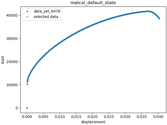
selected_data = synthetic_data[[peak_load_arg]]
selected_data.set_name("selected data")

dc = DataCollection("synthetic", synthetic_data, selected_data)
dc.plot("displacement", "load")

import matplotlib.pyplot as plt
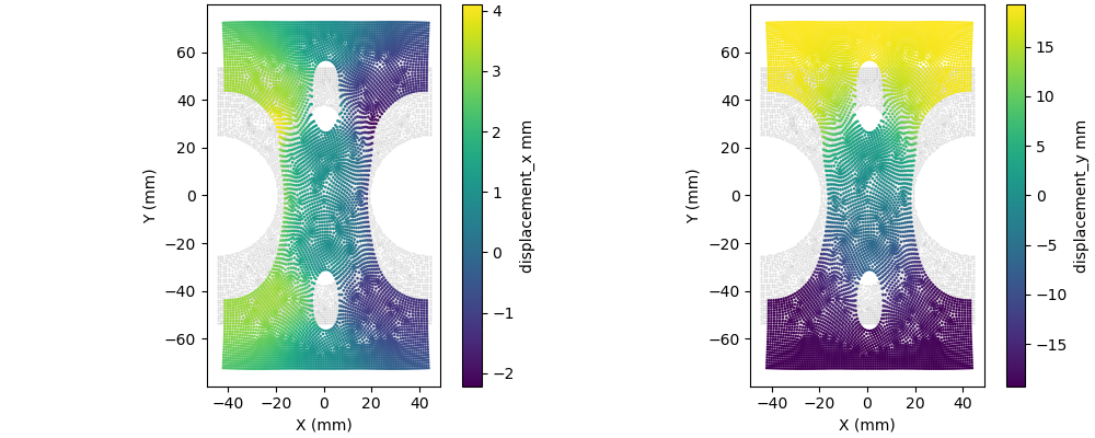
def plot_field(data, field, ax):
    c = ax.scatter(1e3*(data.spatial_coords[:,0]),
                   1e3*(data.spatial_coords[:,1]),
                   c="#bdbdbd", marker='.', s=1, alpha=0.5)
    c = ax.scatter(1e3*(data.spatial_coords[:,0]+data["displacement_x"][-1, :]),
                   1e3*(data.spatial_coords[:,1]+data["displacement_y"][-1, :]),
                   c=1e3*data[field][-1, :], marker='.', s=3)
    ax.set_xlabel("X (mm)")
    ax.set_ylabel("Y (mm)")
    ax.set_aspect('equal')
    fig.colorbar(c, ax=ax, label=f"{field} mm")

fig, axes = plt.subplots(1,2, figsize=(10,4), constrained_layout=True)
plot_field(synthetic_data, "displacement_x", axes[0])
plot_field(synthetic_data, "displacement_y", axes[1])
plt.show()

mat_file_string = """begin material test_material
  density = 1
  begin parameters for model hill_plasticity
    youngs modulus  = {elastic_modulus*1e9}
    poissons ratio  = {poissons}
    yield_stress    = {yield_stress*1e6}

    hardening model = voce
    hardening modulus = {A*1e6}
    exponential coefficient = {n}

    coordinate system = rectangular_coordinate_system

    R11 = {R11}
    R22 = {R22}
    R33 = {R33}
    R12 = {R12}
    R23 = {R23}
    R31 = {R31}
  end
end
"""

with open("modular_plasticity.inc", 'w') as fn:
    fn.write(mat_file_string)


model = UserDefinedSierraModel("adagio", "synthetic_data_files/test_model_input_reduced_output.i",
                               "synthetic_data_files/test_mesh.g", "modular_plasticity.inc")
model.set_name("test_model")
model.add_constants(elastic_modulus=200, poissons=0.27, R22=1.0,
                    R33=0.9, R23=1.0, R31=1.0)
model.read_full_field_data("surf_results.e")
from site_matcal.sandia.computing_platforms import is_sandia_cluster, get_sandia_computing_platform
from site_matcal.sandia.tests.utilities import MATCAL_WCID
num_cores=96
if is_sandia_cluster():
    model.run_in_queue(MATCAL_WCID, 45/60.0)
    model.continue_when_simulation_fails()
    platform = get_sandia_computing_platform()
    num_cores = platform.get_processors_per_node()
model.set_number_of_cores(num_cores)

interpolate_objective = InterpolatedFullFieldObjective("synthetic_data_files/test_mesh_surf.g",
                                                       "displacement_x",
                                                       "displacement_y")
interpolate_objective.set_name("interpolate_objective")

max_load = float(np.max(synthetic_data["load"]))
load_objective = CurveBasedInterpolatedObjective("displacement", "load")
load_objective.set_name("load_objective")

Y = Parameter("yield_stress", 100, 500.0, 200*.96)
A = Parameter("A", 100, 4000, 1500*0.96)
n = Parameter("n", 1, 10, 2*1.04)
R11 = Parameter("R11", 0.8, 1.1, 0.95*0.96)
R12 = Parameter("R12", 0.8, 1.1, 0.85*1.04)

param_collection = ParameterCollection("Hill48 in-plane", Y, A, n, R11, R12)

study = GradientCalibrationStudy(param_collection)
study.set_results_storage_options(results_save_frequency=len(param_collection)+1)
study.set_core_limit(100)
study.add_evaluation_set(model, load_objective, synthetic_data)
study.add_evaluation_set(model, interpolate_objective, selected_data)
study.set_working_directory("ff_interp_cal_success", remove_existing=True)
study.do_not_save_evaluation_cache()
study.set_step_size(1e-4)
results = study.launch()

calibrated_params = results.best.to_dict()
print(calibrated_params)

goal_results = {"yield_stress":200,
                "A":1500,
                "n":2,
                "R11":0.95,
                "R12":0.85}

def pe(result, goal):
    return (result-goal)/goal*100

for param in goal_results.keys():
    print(f"Parameter {param} error: {pe(calibrated_params[param], goal_results[param])}")

• 
• 

Opening exodus file: ../../../docs_support_files/synthetic_surf_results_0_degree.e
Opening exodus file: ../../../docs_support_files/synthetic_surf_results_0_degree.e
Closing exodus file: ../../../docs_support_files/synthetic_surf_results_0_degree.e
Closing exodus file: ../../../docs_support_files/synthetic_surf_results_0_degree.e
Opening exodus file: synthetic_data_files/test_mesh_surf.g
Closing exodus file: synthetic_data_files/test_mesh_surf.g
Opening exodus file: synthetic_data_files/test_mesh_surf.g
Closing exodus file: synthetic_data_files/test_mesh_surf.g
OrderedDict({'yield_stress': 199.99658235, 'A': 1499.9887296, 'n': 2.0000287356, 'R11': 0.95000878217, 'R12': 0.85000757337})
Parameter yield_stress error: -0.0017088249999943628
Parameter A error: -0.0007513600000038423
Parameter n error: 0.0014367799999970288
Parameter R11 error: 0.0009244389473683195
Parameter R12 error: 0.0008909847058839492

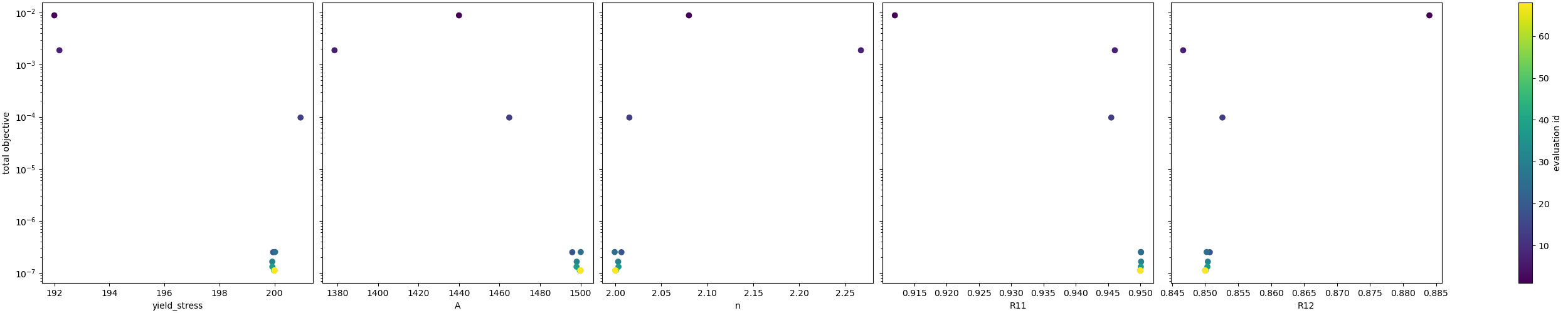
The calibration finishes with RELATIVE FUNCTION CONVERGENCE and the calibrated parameter percent errors are all below 0.1%. A quality solution was obtained through the careful choice of objective and by starting near the global minimum.

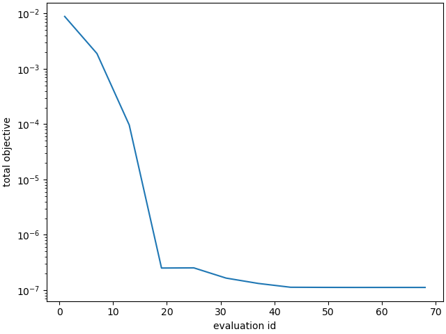
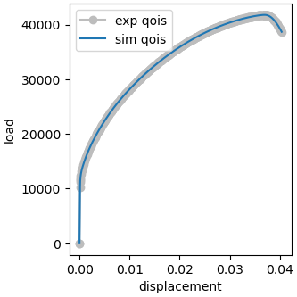
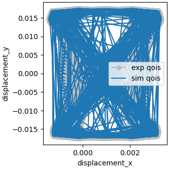
As expected, when we plot the results below, we see that the results for the load-displacement curve agree well with the synthetic data. Both objectives drop quickly to values near 1-e4. The interpolation objective is decreasing at all times and stagnates quickly.

Note

The QoIs are purposefully not plotted for the full-field interpolation objective. This is done to avoid saving and moving the large data sets which can exacerbated out-of-memory issues.

import os
init_dir = os.getcwd()
os.chdir("ff_interp_cal_success")
make_standard_plots("displacement","displacement_x")
os.chdir(init_dir)


# sphinx_gallery_thumbnail_number = 5

• 
• 
• 
•