Model Discrepancy Issue Example

In this case, the data comes from an exponential function with relatively low added noise. The model is a bilinear function producing results similar to an elastic-plastic response with the parameter “Y” controlling where the change from one linear trend to the other takes place and the parameter “H” controlling the slope of the second trend. The slope of the initial trend is fixed, as if it were known (as the elastic modulus typically would be).

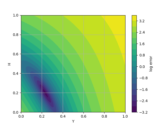
The fit is well defined in the sense that the error contours are closed, and the bowl is steep; however, the model discrepancy and the constraint of fixed E clearly have effects on the fit. For instance, the changeover point in the bilinear “plasticity” model is ambiguous as evidenced by the elongated diagonal error contours. Also extrapolating the fitted model will not follow the data. This issue is common in fitting real material models to data that spans large ranges of, for example, strain, strain-rate and temperature.

To begin the calibration, we import MatCal and Numpy.

from matcal import *
import numpy as np

We create a python function to be used as a MatCal PythonModel for this calibration. The python model uses Numpy in the function and requires that Numpy be imported within the function. As stated above, the data will be fitted to a model with a bilinear response similar to an elastic-plastic model. The initial slope (E) is assumed to be known. The parameter “Y” determines where the model changes to the second linear trend and the parameters “H” determines the second slope.

def bilinear_model(**parameters):
  import numpy as np
  max_strain = 1.0
  npoints = 100
  strain = np.linspace(0,max_strain,npoints)
  E = 1.5
  Y = parameters['Y']
  H = parameters['H']
  eY = Y/E
  stress = np.where(strain < eY, E*strain, Y + H*(strain-eY))
  response = {'strain':strain, 'stress': stress}
  return response

With the function for the model defined above, we create the parameters for our MatCal calibration study and the MatCal PythonModel from the function.

Y = Parameter('Y',0.0,1.0, 0.51)
H = Parameter('H',0.0,1.0, 0.51)
parameters = ParameterCollection('parameters', Y, H)
model = PythonModel(bilinear_model)

A simple gradient-based calibration with a mean squared error objective is enough to illustrate the point. We load the data, create the calibration based on the model parameters, and define an objective for fitting the model response to the data.

data = FileData('exponential.csv')
calibration = GradientCalibrationStudy(parameters)
objective = CurveBasedInterpolatedObjective('strain','stress')
objective.set_name("stress-strain")
calibration.add_evaluation_set(model, objective, data)

We can then run the calibration and select the optimal parameters and the best fit.

results = calibration.launch()
best_parameters = results.best.to_dict()
best_response = results.best_simulation_data(model, 'matcal_default_state')

We also grab the true/experimental response and the model/fitted response

data_strain = data['strain']
data_stress = data['stress']
model_strain = best_response['strain']
model_stress = best_response['stress']

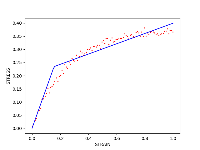
First, compare the response curves. We plot the calibrated model with lines and the data with points. Generally, there are about as many points above the fitted line as below. This is due to using a mean squared error objective but here it causes the fit to miss “features” such as the soft transition from the initial linear trend to the exponential one. Also, since the fit does not emphasize the slope at the end of the data, using this model outside the fitted region will lead to large extrapolation errors, i.e., the model will overestimate the output.

import matplotlib.pyplot as plt
plt.plot(model_strain,model_stress,'b',label="fit")
plt.scatter(data_strain,data_stress,2,'r',label="data")
plt.xlabel("STRAIN")
plt.ylabel("STRESS")

Text(33.722222222222214, 0.5, 'STRESS')

Second, examine how the error changes in the vicinity of the best fit. This a helper function to evaluate the error on a grid of parameter values for plotting. MatCal’s ParameterStudy can also do this.

def sample_error(model, data, ranges = {"Y":[0.0,1.0],"H":[0.0,1.0]} ):
  Ys, Hs = np.mgrid[ ranges["Y"][0]:ranges["Y"][1]:100j, ranges["H"][0]:ranges["H"][1]:100j]
  Zs = np.empty_like(Ys)
  for i in range(Ys.shape[0]):
    for j in range(Ys.shape[1]):
      parameters = {"Y":Ys[i,j],"H":Hs[i,j]}
      response = model(**parameters)
      residual = response['stress']-data['stress']
      error = np.sum(residual**2)
      Zs[i,j] = error
  return Ys,Hs,Zs

The contour plot depicts the change in error in the vicinity of the optimum. Clearly it rises smoothly from the minimum at the optimum. Here, with a nonlinear dependence on the parameters, the bowl does not have perfectly elliptical contours.

Ys,Hs,Zs = sample_error(bilinear_model,data)
plt.contourf(Ys,Hs,np.log(Zs),20)
plt.grid(True)
plt.xlabel("Y")
plt.ylabel("H")
plt.colorbar(label="log error")

<matplotlib.colorbar.Colorbar object at 0x155517b6c950>