Note

Go to the end to download the full example code.

Virtual Fields Method Verification

In this example, we verify the virtual power residual calculation for a boundary value problem (BVP) with an analytical solution. To conform to our VFM implementation constraints, we chose a thin plate of length $H$ loaded in uniaxial tension in the Y direction with a distributed load with an over all magnitude of $L$ . Assuming linear elasticity and small deformation, the stress in the Y direction in the plate is

$\sigma_{yy} =\frac{L}{W T}$

where $W$ is the plate width and $T$ is the plate thickness. All other stresses are zero. The in-plane displacements in the plate are given by

$u=-\nu\frac{\sigma_{yy}}{E}x$

and

$v=\frac{\sigma_{yy}}{E}y$

where $E$ is the material elastic modulus, $\nu$ is the material Poisson’s ratio, and $x$ and $y$ are the locations on the plate.

The internal virtual power becomes

$P_{int}=\frac{L}{Wt}\int_{z=-T/2}^{T/2}\int_{y=-H/2}^{H/2}\int_{x=-W/2}^{W/2}\dot{\mathbf{F}}^*_{yy}dxdydz$

where $\dot{\mathbf{F}}^*_{yy}$ is the $\frac{\partial\mathbf{v}^*}{\partial y}$ . The virtual velocity function used is

$\mathbf{v}^*_y=\frac{2y+H}{2H}$

With this virtual velocity function, the virtual velocity gradient component of interest is

$\frac{\partial\mathbf{v}^*}{\partial y} = 1/h.$

As a result, the internal virtual power is given as

$P_{int}=L$

The external virtual power, as expected, results an equivalent value.

$P_{ext} = L\mathbf{v}^*_y = L\frac{2H/2+H}{2H} = L$

With an analytical solution for the virtual internal and external powers available for the BVP of interest, we will create MatCal VFM objects with the proper input and verify that they return the expect values.

We will begin by creating synthetic data that represents the experimental data for this BVP. To do so, we import MatCal’s tools and create the variables needed for the analytical solutions above. We will need:

The materials elastics constants $E$ and $\nu$ . We choose values that are similar to steel with $E=200$ GPa and $\nu=0.25$ .
The plate dimensions $H=15.2$ mm, $W=7.6$ , and $T=0.1$ mm with a discretization in Y and Y.
The load magnitude as a function of time $L(t)$ . We will choose $L(t)$ such that the maximum stress in the plate is 100 MPa.
The number of time steps and the time values.

from matcal import *
import numpy as np

E = 200e9
nu = 0.25

H = 15.2e-3
W = 7.6e-3
T = 0.1e-3

measured_num_points = 10
measured_xs = np.linspace(0, W, measured_num_points)
measured_ys = np.linspace(0, H, measured_num_points)
measured_x_grid, measured_y_grid = np.meshgrid(measured_xs, measured_ys)


n_time_steps = 10
L = np.linspace(0, 100e6*W*T,n_time_steps).reshape(n_time_steps,1)
time = np.linspace(0,1,n_time_steps)

With all the required inputs initialized, we can create the FieldData objects that are need to have MatCal evaluate the virtual powers for the problem. The FieldData object requires several fields:

time
load
The X locations of the field data
The Y locations of the data
The X displacements for each point (U)
The Y displacements for each point (V)

sigma_yy = L/(W*T)

def displacements(x,y):
    return  -nu*sigma_yy/E*x, sigma_yy/E*y

all_x_1D = measured_x_grid.reshape(measured_num_points**2)
all_y_1D = measured_y_grid.reshape(measured_num_points**2)
u,v = displacements(all_x_1D, all_y_1D)

After creating the values for the fields that we need, they can be combined into a dictionary and converted into a MatCal FieldData object using the convert_dictionary_to_field_data() function.

data_dict = {'time':time, 'load':L,
             "X":all_x_1D,
             "Y":all_y_1D,
             "U":u,
             "V":v}

field_data = convert_dictionary_to_field_data(data_dict,
                                              coordinate_names=["X", "Y"])

Next, a discretization for the VFM models must be created. MatCal has a simple tool for creating rectangular volumes that we will use, the auto_generate_two_dimensional_field_grid() function. It requires the number of X and Y discretization points and the field data that the mesh is intended to encapsulate as inputs. It will return MatCal’s two dimensional mesh class that can be used as a mesh input to MatCal’s VFM model. It currently can only be used for rectangular shapes without holes.

from matcal.full_field.TwoDimensionalFieldGrid import auto_generate_two_dimensional_field_grid
auto_mesh = auto_generate_two_dimensional_field_grid(measured_num_points*5,
                                                     measured_num_points*5, field_data)

The next item needed for the creation of the MatCal VFM models is a SierraSM material file. We will create a simple elastic material model file using Python file tools and then create a MatCal Material object so the VFM models can use that material.

material_file_string = \
"""
  begin material steel
    begin parameters for model elastic
      youngs modulus                =  {E}
      poissons ratio                =   {nu}
    end
  end
"""

with open("elastic_material.inc", "w") as mf:
    mf.write(material_file_string)

material = Material("steel", "elastic_material.inc", "elastic")

We can now create the VFM models that we want to evaluate. We will look at two VFM models, The VFMUniaxialTensionHexModel and the VFMUniaxialTensionConnectedHexModel will both be evaluated in this verification example. The models require a material, a mesh and thickness to be initialized and field data with a two-dimensional displacement field to be added as the boundary condition data. We optionally set the names so their results can be more easily pulled from the results data object returned from our study.

default_hex_model = VFMUniaxialTensionHexModel(material, auto_mesh, T)
default_hex_model.set_name("default_VFM_hex_model")
default_hex_model.add_boundary_condition_data(field_data)
default_hex_model.set_number_of_time_steps(20)

connected_hex_model = VFMUniaxialTensionConnectedHexModel(material, auto_mesh, T)
connected_hex_model.set_name("VFM_connected_hex_model")
connected_hex_model.add_boundary_condition_data(field_data)
connected_hex_model.set_number_of_time_steps(20)

The final step is to create the parameters for the study, the objective to be evaluated and the study itself. For our elastic model, the only parameters we need are the elastic modulus and the Poisson’s ratio. The study we will use to evaluate the models is the ParameterStudy since just need the model results at our predetermined steel-like parameter values. Since this study is evaluating a VFM model, we create a VFM model with no inputs because our global data fields of “time” and “load” match the default ones expected by the objective.

E_param = Parameter('E', 100e9, 300e9)
nu_param = Parameter('nu', 0.1, 0.5)

vfm_objective = MechanicalVFMObjective()
vfm_objective.set_name('vfm_objective')

After creating the parameters, objectives, synthetic data and models, we can create the study and add the evaluation sets and parameter values that we want to evaluate. The study is then launched and the results are stored in an object that we can analyze when the study completes.

study = ParameterStudy(E_param, nu_param)
study.add_parameter_evaluation(E=E, nu=nu)
study.add_evaluation_set(default_hex_model, vfm_objective, field_data)
study.add_evaluation_set(connected_hex_model, vfm_objective, field_data)
study.set_core_limit(3)
results = study.launch()

You are using exodus.py v 1.21.6 (seacas-py3), a python wrapper of some of the exodus library.

Copyright (c) 2013-2023 National Technology &
Engineering Solutions of Sandia, LLC (NTESS).  Under the terms of
Contract DE-NA0003525 with NTESS, the U.S. Government retains certain
rights in this software.

Opening exodus file: matcal_template/default_VFM_hex_model/matcal_default_state/default_VFM_hex_model.g
Closing exodus file: matcal_template/default_VFM_hex_model/matcal_default_state/default_VFM_hex_model.g
Opening exodus file: matcal_template/default_VFM_hex_model/matcal_default_state/default_VFM_hex_model.g
Closing exodus file: matcal_template/default_VFM_hex_model/matcal_default_state/default_VFM_hex_model.g
Opening exodus file: matcal_template/default_VFM_hex_model/matcal_default_state/default_VFM_hex_model.g
Closing exodus file: matcal_template/default_VFM_hex_model/matcal_default_state/default_VFM_hex_model.g
Opening exodus file: matcal_template/default_VFM_hex_model/matcal_default_state/default_VFM_hex_model.g
Opening exodus file: matcal_template/default_VFM_hex_model/matcal_default_state/default_VFM_hex_model_exploded.g
Closing exodus file: matcal_template/default_VFM_hex_model/matcal_default_state/default_VFM_hex_model_exploded.g
Closing exodus file: matcal_template/default_VFM_hex_model/matcal_default_state/default_VFM_hex_model.g
Opening exodus file: matcal_template/VFM_connected_hex_model/matcal_default_state/VFM_connected_hex_model.g
Closing exodus file: matcal_template/VFM_connected_hex_model/matcal_default_state/VFM_connected_hex_model.g
Opening exodus file: matcal_template/VFM_connected_hex_model/matcal_default_state/VFM_connected_hex_model.g
Closing exodus file: matcal_template/VFM_connected_hex_model/matcal_default_state/VFM_connected_hex_model.g
Opening exodus file: matcal_template/VFM_connected_hex_model/matcal_default_state/VFM_connected_hex_model.g
Closing exodus file: matcal_template/VFM_connected_hex_model/matcal_default_state/VFM_connected_hex_model.g

In this verification problem, our goal is to verify that our MatCal VFM objective is accurately evaluating the internal and external virtual powers. As a result, we extract these virtual powers from the study results and compare them to the analytically determined value for the internal power $L\left(t\right)$ . We compare them by evaluating their percent error with the following equation

$Pe = 100\frac{P_{eval} - L}{\max\left(L\right)}$

where $P_{eval}$ is the evaluated virtual power (either the internal or external from either model). Since we will evaluate this percent error several times, we make a function to perform the calculation.

def percent_error(prediction, actual):
    return (prediction - actual)/np.max(actual)*100

We then extract the results from each of the models and print or plot their errors.

matcal_internal_power_default = results.best_simulation_qois(default_hex_model,
                                                             vfm_objective,
                                                             field_data.state,
                                                             0)["virtual_power"]
matcal_external_power_default = results.get_experiment_qois(default_hex_model,
                                                             vfm_objective,
                                                             field_data.state,
                                                             0)["virtual_power"]

matcal_internal_power_connected = results.best_simulation_qois(connected_hex_model,
                                                             vfm_objective,
                                                             field_data.state,
                                                             0)["virtual_power"]
matcal_external_power_connected = results.get_experiment_qois(connected_hex_model,
                                                             vfm_objective,
                                                             field_data.state,
                                                             0)["virtual_power"]

print(percent_error(matcal_external_power_default, L))
print(percent_error(matcal_external_power_connected, L))

[[0.]
 [0.]
 [0.]
 [0.]
 [0.]
 [0.]
 [0.]
 [0.]
 [0.]
 [0.]]
[[0.]
 [0.]
 [0.]
 [0.]
 [0.]
 [0.]
 [0.]
 [0.]
 [0.]
 [0.]]

Both of the external powers have no error. This is expected as our experimental data for this study was exact. This result demonstrates in part that all of the MatCal’s VFM objective calculations and virtual fields are correctly implemented. We have unit tests that test each of the components to contribute to this individually. The next evaluation compares the internal virtual power to the expected virtual power. This is significantly more involved as it requires the simulation of the VFM model using SierraSM.

internal_power_error_default = percent_error(matcal_internal_power_default.reshape(10,1), L)
internal_power_error_connected = percent_error(matcal_internal_power_connected.reshape(10,1), L)
print(internal_power_error_default)
print(internal_power_error_connected)

[[ 0.        ]
 [-0.0006654 ]
 [-0.00260389]
 [-0.00581517]
 [-0.01029905]
 [-0.01608401]
 [-0.02317037]
 [-0.03152879]
 [-0.04115908]
 [-0.05206094]]
[[ 0.        ]
 [-0.0006654 ]
 [-0.00260389]
 [-0.00581517]
 [-0.01029905]
 [-0.01608401]
 [-0.02317037]
 [-0.03152879]
 [-0.04115908]
 [-0.05206094]]

When we print the percent errors, it is clear that the some part of the process has introduced errors. The magnitude of the maximum error is 0.05%. To further investigate, we plot the internal power errors as a function time.

import matplotlib.pyplot as plt

plt.plot(time, internal_power_error_default, label="default VFM model", marker='o')
plt.plot(time, internal_power_error_connected, label="connected hex VFM model")

plt.xlabel("time (s)")
plt.ylabel("Internal Power Error (%)")
plt.legend()
plt.show()

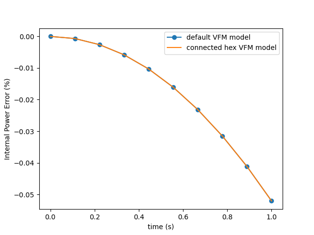
The error is increasing quadratically as the load is increased and the model becomes more deformed. This error is due to our initial assumption of small deformation. SierraSM is formulated as a large deformation code. As a result, our small deformation assumption results in this small, but noticeable error. In later verification examples, we evaluate our methods with synthetic data using large deformation solutions and are able to obtain results with much smaller errors.

Total running time of the script: (2 minutes 1.271 seconds)

Gallery generated by Sphinx-Gallery