Note
Go to the end to download the full example code.
6061T6 aluminum temperature dependent calibration
With our model form chosen and initial point for the calibration determined, we can begin the final calibration for the temperature dependence functions.
Note
Useful Documentation links:
Since the behavior for each temperature is independent, we will actually be performing three subsequent calibrations, one for each temperature. We begin by importing the tools needed for the calibration and setting our default plotting options.
from matcal import *
from site_matcal.sandia.computing_platforms import is_sandia_cluster, get_sandia_computing_platform
from site_matcal.sandia.tests.utilities import MATCAL_WCID

import matplotlib.pyplot as plt
from matplotlib import cm

plt.rc('text', usetex=True)
plt.rc('font', family='serif')
plt.rc('font', size=12)
figsize = (6,4)
Next, we import the data for the calibration. We
only import the high temperature data since
we are only calibrating the temperature
scaling functions as described in the previous
steps from this example suite. We modify the data
after it is imported so that the stress units are in psi
and remove the time field as it is not required
for the boundary condition determination for this calibration.
See Uniaxial tension solid mechanics boundary conditions.
high_temp_data_collection = BatchDataImporter("aluminum_6061_data/"
                                              "uniaxial_tension/processed_data/*6061*.csv",).batch
high_temp_data_collection = scale_data_collection(high_temp_data_collection,
                                                  "engineering_stress", 1000)
high_temp_data_collection.remove_field("time")
We save the states from the data in a variable we will use later when setting up the calibrations.
all_states = high_temp_data_collection.states
Next, we plot the data to verify the data imported as expected.
See
DataCollection and Data Importing and Manipulation
for more information on importing, manipulating and storing data in MatCal.
Because MatCal is a Python library, you can still use all the existing Python tools and features
to manipulate data and Python objects. Here we create functions that perform the plotting
that we want to do for each temperature and then call these functions to
create the plots we want.
First, we create a function that determines colors
for data in a data collection
using the RdYlBu color map. Using this function, colors
are set such that
cooler temperatures are blue and higher temperatures are red
over the temperature range that we have data (533 - 1032 R).
cmap = cm.get_cmap("RdYlBu")
def get_colors(bc_data_dc):
    colors = {}
    for state_name in bc_data_dc.state_names:
        temp = bc_data_dc.states[state_name]["temperature"]
        colors[temp] = cmap(1.0-(temp-533.0)/(1032.0-533.0))
    return colors
colors = get_colors(high_temp_data_collection)
/gpfs/knkarls/projects/matcal-stable/external_matcal/documentation/advanced_examples/6061T6_anisotropic_calibration/plot_6061T6_f_temperature_dependent_calibration_cluster.py:73: MatplotlibDeprecationWarning: The get_cmap function was deprecated in Matplotlib 3.7 and will be removed two minor releases later. Use ``matplotlib.colormaps[name]`` or ``matplotlib.colormaps.get_cmap(obj)`` instead.
  cmap = cm.get_cmap("RdYlBu")
This next function plots each direction for a given temperature on a provided figure with colors and options as desired.
def plot_directions_for_temp(temp_str, fig):
    temp = float(temp_str)
    high_temp_data_collection.plot("engineering_strain", "engineering_stress", figure=fig,
                                    show=False, state=f"temperature_{temp_str}_direction_R22",
                                    color=colors[temp], labels=f"R22, {temp:0.0f} R",
                                    linestyle="-")
    high_temp_data_collection.plot("engineering_strain", "engineering_stress", figure=fig,
                                    show=False, state=f"temperature_{temp_str}_direction_R11",
                                    color=colors[temp], labels=f"R11, {temp:0.0f} R",
                                    linestyle="--")
    high_temp_data_collection.plot("engineering_strain", "engineering_stress", figure=fig,
                                    show=False, state=f"temperature_{temp_str}_direction_R33",
                                    color=colors[temp], labels=f"R33, {temp:0.0f} R",
                                    linestyle=":")
With our plotting functions created, we create a figure and then call the plotting function with the appropriate data passed to it.
all_data_fig = plt.figure("high temperature data", figsize=figsize, constrained_layout=True)
plot_directions_for_temp("6.716700e+02", all_data_fig)
plot_directions_for_temp("8.516700e+02", all_data_fig)
plot_directions_for_temp("1.031670e+03", all_data_fig)
plt.xlabel("engineering strain ()")
plt.ylabel("engineering stress (psi)")
plt.show()
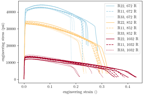
In the plot, we can see the data imported as expected and is ready to be used in the calibration.
We now setup the material model files
needed for the calibration and create
the MatCal Parameter
objects that must be calibrated for this material
model.
First, we create the material model
input file that is needed by MatCal and SIERRA/SM
for the RoundUniaxialTensionModel
that will be used in this calibration. We will
do this using Python’s string and
file tools. Before creating the
string that will be written as
the material model input deck,
we create some variables that will be
used in the string.
material_model = "hill_plasticity"
material_name = "ductile_failure_6061T6"
density = 0.0975/(32.1741*12)
youngs_modulus=10.3e6
poissons_ratio=0.33
With the constants defined above, we can create the material model input deck string. This is a modified version of the file from 6061T6 aluminum calibration with anisotropic yield with the addition of temperature dependent functions for the yield and Voce hardening parameters.
material_file_string = f"""
  begin definition for function al6061T6_yield_temp_dependence
    type is piecewise linear
    begin values
         533.07, 1
         671.67,  {{Y_scale_factor_672}}
         851.67,  {{Y_scale_factor_852}}
        1031.67, {{Y_scale_factor_1032}}
        1391.67, 0.01
    end
  end

  begin definition for function al6061T6_hardening_mod_temp_dependence
    type is piecewise linear
    begin values
         533.07, 1
         671.67,  {{A_scale_factor_672}}
         851.67,  {{A_scale_factor_852}}
        1031.67, {{A_scale_factor_1032}}
        1391.67, 0.01
    end
  end

  begin definition for function al6061T6_hardening_exp_coeff_temp_dependence
    type is piecewise linear
    begin values
         533.07, 1
         671.67,  {{b_scale_factor_672}}
         851.67,  {{b_scale_factor_852}}
        1031.67, {{b_scale_factor_1032}}
        1391.67, 0.01
    end
  end

  begin material {material_name}
    density = {density}
    begin parameters for model {material_model}
      poissons ratio                = {poissons_ratio}
      youngs modulus                = {youngs_modulus}

      yield stress                  = {{yield_stress*1e3}}
      yield stress function = al6061T6_yield_temp_dependence

      r11                           =   1
      r22                           =   {{R22}}
      r33                           =   {{R33}}
      r12                           =   {{R12}}
      r23                           =   {{R23}}
      r31                           =   {{R31}}
      coordinate system             =   rectangular_coordinate_system

      {{if(direction=="R11")}}
      direction for rotation        = 3
      alpha                         = 90.0
      {{elseif((direction=="R33") || (direction=="R31"))}}
      direction for rotation        = 1
      alpha                         = -90.0
      {{elseif(direction=="R23")}}
      direction for rotation        = 2
      alpha                         = 90.0
      {{endif}}

      hardening model = flow_stress_parameter
      isotropic hardening model = voce_parameter

      hardening modulus = {{hardening*1e3}}
      hardening modulus function = al6061T6_hardening_mod_temp_dependence

      exponential coefficient = {{b}}
      exponential coefficient function = al6061T6_hardening_exp_coeff_temp_dependence

      rate multiplier = rate_independent
    end
  end
"""
Next, we write the string to a file, so MatCal can import it and add it to the models.
material_filename = "hill_plasticity_temperature_dependent.inc"
with open(material_filename, 'w') as fn:
    fn.write(material_file_string)
Then, we create the Material
object that will be used by the
RoundUniaxialTensionModel
to correctly assign the material to the finite element model.
sierra_material = Material(material_name, material_filename, material_model)
Now we create the 9 MatCal parameters that will be calibrated for the material model setup above. We use the estimates for the parameters from 6061T6 aluminum temperature calibration initial point estimation as the initial points for the calibration. We define them as variable below.
temp_param_ips = matcal_load("temperature_parameters_initial.serialized")
y_scale_factor_672_ip = temp_param_ips["Y_scale_factor_672"]
y_scale_factor_852_ip = temp_param_ips["Y_scale_factor_852"]
y_scale_factor_1032_ip = temp_param_ips["Y_scale_factor_1032"]

A_scale_factor_672_ip = temp_param_ips["A_scale_factor_672"]
A_scale_factor_852_ip = temp_param_ips["A_scale_factor_852"]
A_scale_factor_1032_ip = temp_param_ips["A_scale_factor_1032"]

b_scale_factor_672_ip = temp_param_ips["b_scale_factor_672"]
b_scale_factor_852_ip = temp_param_ips["b_scale_factor_852"]
b_scale_factor_1032_ip = temp_param_ips["b_scale_factor_1032"]
Since yield is relatively well characterized using MatFit, we create the parameters for the yield function with fairly close bounds and the current value set to the initial point estimate from the previous example.
Y_scale_factor_672  = Parameter("Y_scale_factor_672", 0.85, 1, y_scale_factor_672_ip)
Y_scale_factor_852  = Parameter("Y_scale_factor_852", 0.45, 0.85, y_scale_factor_852_ip)
Y_scale_factor_1032 = Parameter("Y_scale_factor_1032", 0.05, 0.45, y_scale_factor_1032_ip)
The hardening parameter initial guesses are likely less optimal. As a result, we set the bounds fairly wide for these parameters and again set the current value as the initial point estimate from the previous example.
A_scale_factor_672  = Parameter("A_scale_factor_672", 0.0,
                                2*A_scale_factor_672_ip, A_scale_factor_672_ip)
A_scale_factor_852  = Parameter("A_scale_factor_852", 0.0,
                                2*A_scale_factor_852_ip, A_scale_factor_852_ip)
A_scale_factor_1032 = Parameter("A_scale_factor_1032", 0.0,
                                2*A_scale_factor_1032_ip, A_scale_factor_1032_ip)

b_scale_factor_672  = Parameter("b_scale_factor_672", 0.1,
                                2*b_scale_factor_672_ip, b_scale_factor_672_ip)
b_scale_factor_852  = Parameter("b_scale_factor_852", 0.1,
                                2*b_scale_factor_852_ip, b_scale_factor_852_ip)
b_scale_factor_1032 = Parameter("b_scale_factor_1032", 0.1,
                                2*b_scale_factor_1032_ip, b_scale_factor_1032_ip)
With the parameters, material model and data available,
we can create the RoundUniaxialTensionModel
that will be calibrated to the data.
First, we define the geometry and mesh discretization options for the model.
These parameters are saved in a dictionary that will
be passed into the model initialization function.
gauge_radius = 0.125
element_size = gauge_radius/8
geo_params = {"extensometer_length": 0.5,
               "gauge_length": 0.75,
               "gauge_radius": gauge_radius,
               "grip_radius": 0.25,
               "total_length": 3.2,
               "fillet_radius": 0.25,
               "taper": 0.0015,
               "necking_region":0.375,
               "element_size": element_size,
               "mesh_method":3,
               "grip_contact_length":0.8}
With the geometry defined, we can create the model and, if desired, assign a name.
model = RoundUniaxialTensionModel(sierra_material, **geo_params)
model.set_name("tension_model")
In order for the model to run for each state, we must pass boundary condition information to the model.
model.add_boundary_condition_data(high_temp_data_collection)
To save some simulation time, we apply an allowable load drop factor. Since at high temperatures the test data unloads significantly, we conservatively set the allowable load drop factor to 0.7. This will kill the simulation after its load has dropped 70% from peak load.
model.set_allowable_load_drop_factor(0.70)
We now set computer platform options for this model. Since we may run this example on HPC clusters or non-HPC computers, we determine the platform and choose the platform options accordingly.
if is_sandia_cluster():
    platform = get_sandia_computing_platform()
    model.set_number_of_cores(platform.get_processors_per_node())
    model.run_in_queue(MATCAL_WCID, 0.5)
    model.continue_when_simulation_fails()
else:
    model.set_number_of_cores(8)
We finish the model by adding model constants to the model. For this calibration, the model constants are the calibrated material parameters from 6061T6 aluminum calibration with anisotropic yield
RT_calibrated_params = matcal_load("anisotropy_parameters.serialized")
model.add_constants(**RT_calibrated_params)
Next, we define the objective for the calibration.
We will use the CurveBasedInterpolatedObjective
for this calibration to calibrate to the material
engineering stress/strain curves.
objective = CurveBasedInterpolatedObjective("engineering_strain", "engineering_stress")
To help ensure a successful calibration,
we create a function to be used as a
UserFunctionWeighting
residual weighting object. The function below
will effectively remove the elastic region data
and high strain data where failure is likely from the calibration.
It does this by setting the residuals in these regions to zero.
Since these regions vary somewhat by state, we can access state
variables from the residuals and perform our NumPy
slicing differently according to state. In this case,
the state temperature is used to inform
where the residuals should be set to zero.
def remove_uncalibrated_data_from_residual(engineering_strains, engineering_stresses,
                                           residuals):
    import numpy as np
    weights = np.ones(len(residuals))
    min_strains = {671.67:0.006, 851.67:0.0055, 1031.67:0.0025}
    max_strains = {671.67:0.18, 851.67:0.2, 1031.67:0.2}
    temp=residuals.state["temperature"]
    weights[engineering_strains < min_strains[temp]] = 0
    weights[engineering_strains > max_strains[temp]] = 0
    return weights*residuals
With the weighting function created,
we create the UserFunctionWeighting
object and add it to the objective.
residual_weights = UserFunctionWeighting("engineering_strain", "engineering_stress",
                                          remove_uncalibrated_data_from_residual)
objective.set_field_weights(residual_weights)
We are now ready to create and run our calibration
studies. As stated previously,
we will perform an independent calibration
for each temperature. For each temperature,
we calibrate to each direction. Although
we would have a successful calibration only
calibrating to the  direction, it is important
that we find a true local minima with all data of interest.
This local minima is required to support our follow-on uncertainty quantification
activity with a
direction, it is important
that we find a true local minima with all data of interest.
This local minima is required to support our follow-on uncertainty quantification
activity with a LaplaceStudy.
Each calibration uses
a GradientCalibrationStudy.
We initialize the study with the parameters governing the behavior for the
temperature of interest.
calibration = GradientCalibrationStudy(Y_scale_factor_672, A_scale_factor_672,
                                       b_scale_factor_672)
Next, we create a StateCollection
including only the states desired for the current temperature.
temp_672_states = StateCollection("temp 672 states",
                                  all_states["temperature_6.716700e+02_direction_R11"],
                                  all_states["temperature_6.716700e+02_direction_R22"],
                                  all_states["temperature_6.716700e+02_direction_R33"])
We then add an evaluation set with our desired model, objective, data and the states of interest for this calibration.
calibration.add_evaluation_set(model, objective, high_temp_data_collection,
                               temp_672_states)
We finish the calibration setup by setting the number of cores for the calibration, and assigning a work directory subfolder for the calibration.
if is_sandia_cluster():
    calibration.set_core_limit(4*3+1)
else:
    calibration.set_core_limit(60)
calibration.set_working_directory("672R_calibration", remove_existing=True)
The calibration is run and the results are saved to be plotted when all calibrations are complete.
temp_672_results = calibration.launch()
all_results = temp_672_results.best.to_dict()
The model is then updated to include model constants from the calibration results.
model.add_constants(**all_results)
The two remaining calibrations are setup and run the same way.
calibration = GradientCalibrationStudy(Y_scale_factor_852, A_scale_factor_852,
                                       b_scale_factor_852)

temp_852_states = StateCollection("temp 852 states",
                                  all_states["temperature_8.516700e+02_direction_R11"],
                                  all_states["temperature_8.516700e+02_direction_R22"],
                                  all_states["temperature_8.516700e+02_direction_R33"])

calibration.add_evaluation_set(model, objective, high_temp_data_collection,
                               temp_852_states)
if is_sandia_cluster():
    calibration.set_core_limit(4*3+1)
else:
    calibration.set_core_limit(60)
calibration.set_working_directory("852R_calibration", remove_existing=True)
temp_852_results = calibration.launch()
all_results.update(temp_852_results.best.to_dict())
model.add_constants(**all_results)

temp_1032_states = StateCollection("temp 1032 states",
                                  all_states["temperature_1.031670e+03_direction_R11"],
                                  all_states["temperature_1.031670e+03_direction_R22"],
                                  all_states["temperature_1.031670e+03_direction_R33"])
calibration = GradientCalibrationStudy(Y_scale_factor_1032, A_scale_factor_1032,
                                       b_scale_factor_1032)
calibration.add_evaluation_set(model, objective, high_temp_data_collection,
                               temp_1032_states)
if is_sandia_cluster():
    calibration.set_core_limit(4*3+1)
else:
    calibration.set_core_limit(60)
calibration.set_working_directory("1032R_calibration", remove_existing=True)
temp_1032_results = calibration.launch()
all_results.update(temp_1032_results.best.to_dict())
matcal_save("temperature_dependent_parameters.serialized", all_results)
With all the calibrations completed, we can plot the final temperature dependence function for each parameter and the calibrated material model with the data for each state. First, we extract and organize the calibrated parameters values from the calibration results.
y_temp_dependence = [1,
                     all_results["Y_scale_factor_672"],
                     all_results["Y_scale_factor_852"],
                     all_results["Y_scale_factor_1032"]]
A_temp_dependence = [1,
                     all_results["A_scale_factor_672"],
                     all_results["A_scale_factor_852"],
                     all_results["A_scale_factor_1032"]]
b_temp_dependence = [1,
                     all_results["b_scale_factor_672"],
                     all_results["b_scale_factor_852"],
                     all_results["b_scale_factor_1032"]]

print(y_temp_dependence)
print(A_temp_dependence)
print(b_temp_dependence)
[1, 0.93311096465, 0.78391735862, 0.29237817182]
[1, 0.74204985974, 0.20815247653, 0.071345901932]
[1, 1.2367852356, 1.0123458802, 5.1355335093]
We then organize the initial point estimates similarly for a comparison to the calibrated values.
y_temp_dependence_ip = [1, y_scale_factor_672_ip, y_scale_factor_852_ip,
                         y_scale_factor_1032_ip]
A_temp_dependence_ip = [1, A_scale_factor_672_ip, A_scale_factor_852_ip,
                         A_scale_factor_1032_ip]
b_temp_dependence_ip = [1, b_scale_factor_672_ip, b_scale_factor_852_ip,
                         b_scale_factor_1032_ip]
Now, we plot the functions as we did in 6061T6 aluminum temperature calibration initial point estimation.
temperatures = [533, 672, 852, 1032]
plt.figure()
plt.plot(temperatures, y_temp_dependence, label='yield stress', color="tab:blue")
plt.plot(temperatures, y_temp_dependence_ip, label='yield stress initial',
color="tab:blue", linestyle="--")
plt.plot(temperatures, A_temp_dependence, label='Voce hardening modulus',
color="tab:orange")
plt.plot(temperatures, A_temp_dependence_ip, label='Voce hardening modulus initial',
color="tab:orange", linestyle="--")
plt.plot(temperatures, b_temp_dependence, label='Voce exponential coefficient',
color="tab:green")
plt.plot(temperatures, b_temp_dependence_ip, label='Voce exponential coefficient initial',
color="tab:green", linestyle="--")
plt.ylabel("temperature scaling function (.)")
plt.xlabel("temperature (R)")
plt.legend()
plt.show()
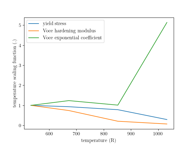
temperatures = [533, 672, 852, 1032]
plt.figure()
plt.plot(temperatures, y_temp_dependence, label='yield stress',
color="tab:blue")
plt.plot(temperatures, A_temp_dependence, label='Voce hardening modulus',
color="tab:orange")
plt.plot(temperatures, b_temp_dependence, label='Voce exponential coefficient',
color="tab:green")
plt.ylabel("temperature scaling function (.)")
plt.xlabel("temperature (R)")
plt.legend()
plt.show()
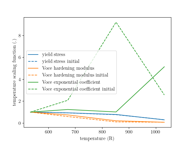
From these plots, we can see that the calibration changed the Voce exponent parameters significantly from the initial point while the yield and Voce saturation stress were only slightly adjusted. As expected and desired, the yield and saturation stress are monotonically decreasing as the temperature increases. However, the Voce exponent decreases before increasing sharply and does not monotonically increase or decrease as the temperature changes. In the next example 6061T6 aluminum temperature dependence verification, we will investigate whether this causes any issues for temperatures between the temperatures to which the model was calibrated.
Next, we compare the calibrated model against the data.
best_indx_672 = temp_672_results.best_evaluation_index
sim_hist_672 = temp_672_results.simulation_history[model.name]

best_indx_852 = temp_852_results.best_evaluation_index
sim_hist_852 = temp_852_results.simulation_history[model.name]

best_indx_1032 = temp_1032_results.best_evaluation_index
sim_hist_1032 =  temp_1032_results.simulation_history[model.name]

def plot_comparison_by_temperature(temp_str, eval_data, best_index):
    fig = plt.figure(f"{temp_str} results", figsize=figsize, constrained_layout=True)
    high_temp_data_collection.plot("engineering_strain", "engineering_stress",
                                   state=f"temperature_{temp_str}_direction_R22",
                                   show=False, figure=fig,
                                   color="tab:red", alpha=0.33,
                                   labels="$R_{22}$ direction data",
                                   markevery=0.01)
    high_temp_data_collection.plot("engineering_strain", "engineering_stress",
                                   state=f"temperature_{temp_str}_direction_R11",
                                   show=False, figure=fig,
                                   color="tab:blue", alpha=0.33,
                                   labels="$R_{11}$ direction data",
                                   markevery=0.01)
    high_temp_data_collection.plot("engineering_strain", "engineering_stress",
                                   state=f"temperature_{temp_str}_direction_R33",
                                   show=False, figure=fig,
                                   color="tab:green", alpha=0.33,
                                   labels="$R_{33}$ direction data",
                                   markevery=0.01)
    data = eval_data[f"temperature_{temp_str}_direction_R22"][best_index]
    plt.plot(data["engineering_strain"], data["engineering_stress"],
             color="tab:red", label="$R_{22}$ direction sim")
    data = eval_data[f"temperature_{temp_str}_direction_R11"][best_index]
    plt.plot(data["engineering_strain"], data["engineering_stress"],
             color="tab:blue", label="$R_{11}$ direction sim")
    data = eval_data[f"temperature_{temp_str}_direction_R33"][0]
    plt.plot(data["engineering_strain"], data["engineering_stress"],
             color="tab:green", label="$R_{33}$ direction sim")
    plt.xlabel("engineering strain (.)")
    plt.ylabel("engineering stress (psi)")
    plt.legend()
    plt.show()

plot_comparison_by_temperature("6.716700e+02", sim_hist_672, best_indx_672)
plot_comparison_by_temperature("8.516700e+02", sim_hist_852, best_indx_852)
plot_comparison_by_temperature("1.031670e+03", sim_hist_1032, best_indx_1032)
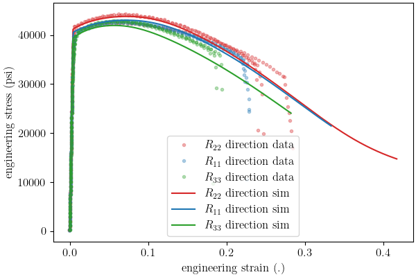
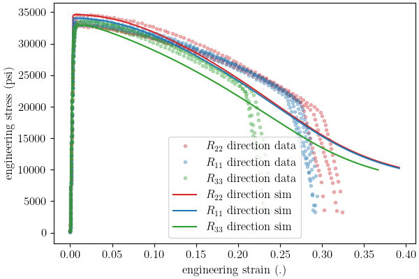
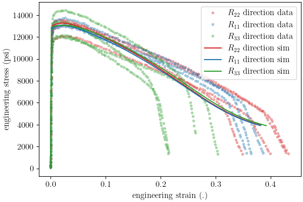
From these plots, we can see that the calbirated models match the experimental data well for each direction and even perform well after strains of 0.2 where the model is technically not calibrated.
Total running time of the script: (37 minutes 55.315 seconds)