6061T6 aluminum temperature dependent data analysis

With the room temperature anisotropic yield model parameterized for this material (see 6061T6 aluminum calibration with anisotropic yield), we now investigate the material’s temperature dependence. Primarily, we are concerned about the following:

1. How the material anisotropy is affected by temperature.

2. How the material plasticity is affected by temperature.

Note

Useful Documentation links:

1. BatchDataImporter

2. plot()

We will investigate these two issues by plotting material features by temperature. The features we are concerned with are the 0.2% offset yield stress, the ultimate stress, the strain at the ultimate stress and the failure strain.

We begin by importing the tools we need to perform this analysis which includes our MatCal tools, NumPy, and matplotlib. We also setup our our plotting defaults.

import numpy as np
from matcal import *
import matplotlib.pyplot as plt
# sphinx_gallery_thumbnail_number = 3
plt.rc('text', usetex=True)
plt.rc('font', family='serif')
plt.rc('font', size=12)
figsize = (4,3)

With our tools imported, we now import the data of interest. Similar to the data import in 6061T6 aluminum data analysis, we import the data using our BatchDataImporter which assigns states to the file according to the state data prepopulated in the data files.

tension_data_collection = BatchDataImporter("aluminum_6061_data/"
                                              "uniaxial_tension/processed_data/cleaned_[CANM]*.csv",).batch
high_temp_data_collection = BatchDataImporter("aluminum_6061_data/"
                                              "uniaxial_tension/processed_data/*6061*.csv",).batch
all_data = tension_data_collection+high_temp_data_collection

Once the data is imported, we perform some data preprocessing which includes scaling the data to be in psi units and removing the unnecessary time field.

all_data = scale_data_collection(all_data, "engineering_stress", 1000)
all_data.remove_field("time")

Since the states are automatically generated, we store the states in variable for later use.

all_states = all_data.states

Next, we plot the data that we will analyze. Since we are interested in its anisotropy and temperature dependence, we will plot all data on one figure. Using MatCal’s plot() method, we can organize, label and mark the different data sets on the plot in a useful manner. Because MatCal is a Python library, you can use all the existing Python tools and features to manipulate data and Python objects. Here we create a function that performs the plotting that we want to do for each temperature.

def plot_directions_for_temp(temp, fig, linestyle):
    all_data.plot("engineering_strain", "engineering_stress", figure=fig,
                   show=False, state=f"temperature_{temp}_direction_R22",
                   color='tab:red', labels=f"R22, {float(temp):0.0f} R",
                   linestyle=linestyle)
    all_data.plot("engineering_strain", "engineering_stress", figure=fig,
                   show=False, state=f"temperature_{temp}_direction_R11",
                   color='tab:blue', labels=f"R11, {float(temp):0.0f} R",
                   linestyle=linestyle)
    all_data.plot("engineering_strain", "engineering_stress", figure=fig,
                   show=False, state=f"temperature_{temp}_direction_R33",
                   color='tab:green', labels=f"R33, {float(temp):0.0f} R",
                   linestyle=linestyle)

With our plotting function created, we create a figure and then call the plotting function with the appropriate data passed to it.

all_data_fig = plt.figure("all data", figsize=(6,4))
plot_directions_for_temp("5.330700e+02", all_data_fig, '-')
plot_directions_for_temp("6.716700e+02", all_data_fig, '--')
plot_directions_for_temp("8.516700e+02", all_data_fig, '-.')
plot_directions_for_temp("1.031670e+03", all_data_fig, ':')
plt.show()

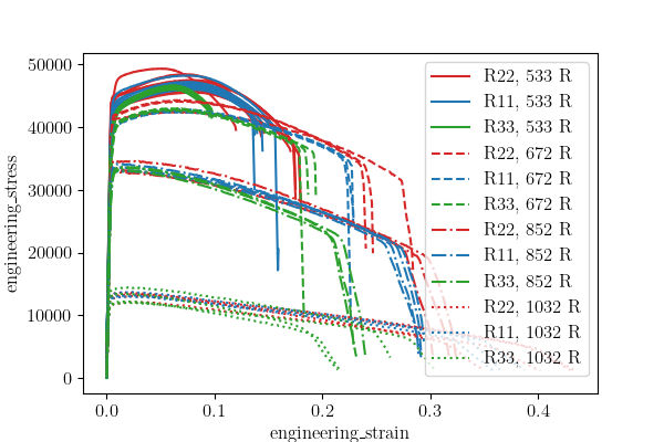
The resulting figure shows each temperature plotted with the different directions clearly identified. The overall stress strain behavior is clearly temperature dependent over this temperature range with the yield and hardening changing significantly as the temperature increases. Qualitatively it appears that the anisotropy is fairly constant through the lower temperatures, however, the trends are not clearly identified by this plot. As a result, we will quantitatively assess the anisotropy with box-and-whisker plots as we did in 6061T6 aluminum data analysis.

First, we must extract the quantities we need for the box-and-whisker plots from the stress strain curves. We extract the yield stress using determine_pt2_offset_yield(). The ultimate stress is determined using NumPy tools and NumPy array slicing. We apply these to the data by looping over each state in the data collection and applying them to each data set in each state.

We store the values in dictionaries according to state to aid in the box-and-whisker plot creature. We create and use a function to update the dictionary for each state since we will be doing this multiple times for each metric of interest.

def save_state_data(data_dict, state_name, data_value):
    if state_name in data_dict:
        data_dict[state_name].append(data_value)
    else:
        data_dict.update({state_name:[data_value]})

    return data_dict

To guarantee order for plotting purposes, we will store the values in ordered dictionaries that will save the data in the order that it is added.

from collections import OrderedDict
yield_stresses = OrderedDict()
ult_stresses = OrderedDict()
strains_at_ult_stresses = OrderedDict()
fail_strains = OrderedDict()

We then create a list from that state names that is ordered according to how we would like the data displayed in the box-and-whisker plots. We arrange the data by increasing temperature and then by the direction so the temperature and direction dependencies can be easily interpreted.

print(all_states.keys())
ordered_state_names = [
    'temperature_5.330700e+02_direction_R11',
    'temperature_5.330700e+02_direction_R22',
    'temperature_5.330700e+02_direction_R33',
    'temperature_6.716700e+02_direction_R11',
    'temperature_6.716700e+02_direction_R22',
    'temperature_6.716700e+02_direction_R33',
    'temperature_8.516700e+02_direction_R11',
    'temperature_8.516700e+02_direction_R22',
    'temperature_8.516700e+02_direction_R33',
    'temperature_1.031670e+03_direction_R11',
    'temperature_1.031670e+03_direction_R22',
    'temperature_1.031670e+03_direction_R33']

odict_keys(['temperature_6.716700e+02_direction_R22', 'temperature_1.031670e+03_direction_R22', 'temperature_8.516700e+02_direction_R22', 'temperature_8.516700e+02_direction_R11', 'temperature_6.716700e+02_direction_R11', 'temperature_1.031670e+03_direction_R11', 'temperature_8.516700e+02_direction_R33', 'temperature_6.716700e+02_direction_R33', 'temperature_1.031670e+03_direction_R33', 'temperature_5.330700e+02_direction_R11', 'temperature_5.330700e+02_direction_R22', 'temperature_5.330700e+02_direction_R33'])

With the data storage objects available, we now loop over the data and extract our metrics for the data analysis.

for state_name in ordered_state_names:
    for data in all_data[state_name]:
        yield_pt = determine_pt2_offset_yield(data, 10e6)
        yield_stress = yield_pt[1]
        yield_stresses = save_state_data(yield_stresses, state_name, yield_stress)
        ult_stress_arg = np.argmax(data["engineering_stress"])
        ult_stress = data["engineering_stress"][ult_stress_arg]
        ult_stresses = save_state_data(ult_stresses, state_name, ult_stress)

        strain_at_ult_stress = data["engineering_strain"][ult_stress_arg]
        strains_at_ult_stresses = save_state_data(strains_at_ult_stresses,
                                                  state_name, strain_at_ult_stress)

        fail_strain = data["engineering_strain"][-1]
        fail_strains = save_state_data(fail_strains, state_name, fail_strain)

To appropriately judge the anisotropy at each temperature, we normalize the stress values by the average of the values for each quantity. A simple function is written to perform this normalization.

def normalize_data(dataset):
    normalized_data = OrderedDict()
    for temp in ["5.330700e+02", "6.716700e+02", "8.516700e+02", "1.031670e+03"]:
        normalizing_state = f"temperature_{temp}_direction_R11"
        normalizing_constant = np.average(dataset[normalizing_state])
        for direction in ["R11", "R22", "R33"]:
            active_state = f"temperature_{temp}_direction_{direction}"
            normalized_values = [val/normalizing_constant for val in dataset[active_state]]
            normalized_data[active_state] = normalized_values
    return normalized_data

normalized_yield_stresses = normalize_data(yield_stresses)
normalized_ult_stresses = normalize_data(ult_stresses)

Now we make the box-and-whisker plots with the appropriate labels. First we plot the yield stresses.

boxplot_labels = [
    "$R_{11}$, 533 R",
    "$R_{22}$, 533 R",
    "$R_{33}$, 533 R",
    "$R_{11}$, 672 R",
    "$R_{22}$, 672 R",
    "$R_{33}$, 672 R",
    "$R_{11}$, 852 R",
    "$R_{22}$, 852 R",
    "$R_{33}$, 852 R",
    "$R_{11}$, 1032 R",
    "$R_{22}$, 1032 R",
    "$R_{33}$, 1032 R",
    ]
plt.figure(constrained_layout=True)
plt.boxplot(normalized_yield_stresses.values(), labels=boxplot_labels)
plt.xlabel("direction")
plt.xticks(rotation=90)
plt.ylabel("normalized yield stress (.)")
plt.show()

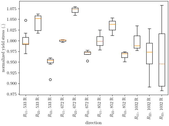
The plot above shows that for the lower temperatures the yield anisotropy remains relatively consistent. Only at the highest temperature does the anisotropy appear to change, but this change is accompanied by a large amount of uncertainty. The normalized ultimate stresses are plotted next.

plt.figure(constrained_layout=True)
plt.boxplot(normalized_ult_stresses.values(), labels=boxplot_labels)
plt.xlabel("direction")
plt.xticks(rotation=90)
plt.ylabel("normalized ultimate stress (.)")
plt.show()

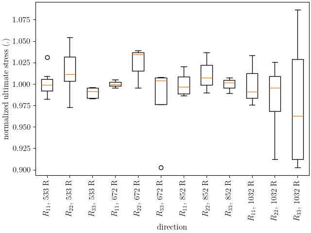
This plot shows that the ultimate stress behavior is similar to the yield stress. As noted in 6061T6 aluminum data analysis, the anisotropy is generally less prominent higher strains for this material indicating anisotropic hardening. We will continue to ignore anisotropic hardening for this example for simplicity.

Next, we plot the strains at the ultimate stress and the failure strains of the data on box-and-whisker plots.

plt.figure(constrained_layout=True)
plt.boxplot(strains_at_ult_stresses.values(), labels=boxplot_labels)
plt.xlabel("direction")
plt.xticks(rotation=90)
plt.ylabel("strain at ultimate stress (.)")
plt.show()

plt.figure(constrained_layout=True)
plt.boxplot(fail_strains.values(), labels=boxplot_labels)
plt.xlabel("direction")
plt.xticks(rotation=90)
plt.ylabel("failure strains (.)")
plt.show()

• 
• 

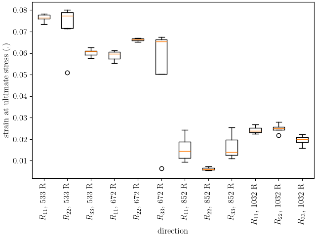
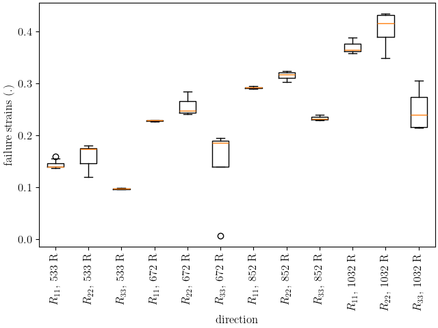
These two plots show that the hardening is significantly affected by temperature as expected. The material increases in ductility and reaches its ultimate stress more quickly as the temperature increases.

With the above plots as guidance, we choose to model the material with the anisotropy calibrated to only the room temperature data. The base material model parameters at room temperature (533 R) will come from 6061T6 aluminum calibration with anisotropic yield. However, this fit will be modified so that the yield and hardening parameters will include temperature dependence. Essentially, the yield and Voce hardening parameters will vary as a function of temperature. They will be given a piecewise-linear temperature dependence where the values will be calibrated at each temperature the material was tested and linear interpolation will be used to predict behavior between this temperatures.

In 6061T6 aluminum temperature calibration initial point estimation, we calculate initial estimates for these functions using MatFit. To support this, we save the data required to use MatFit. We use the function below to save the yield stresses, ultimate stresses, strains at ultimate stress and failure strains for each data set in a file for each state.

for state in yield_stresses:
    zipped_data = zip(yield_stresses[state],
                      ult_stresses[state],
                      strains_at_ult_stresses[state],
                      fail_strains[state])
    with open(f"{state}_matfit_metrics.csv", "w") as file_handle:
        file_handle.write("yield_stress, ultimate_stress, "
                          "strain_at_ultimate_stress, failure_strain\n")
        for yield_str, ult_str, strain_at_ult, fail_strain in zipped_data:
            file_handle.write(f"{yield_str}, {ult_str}, {strain_at_ult}, {fail_strain}\n")