Full-field Interpolation Verification

In this example, we use an analytical function to test and verify our use and implementation of the Compadre GMLS algorithm. We design the verification problem to be representative of the full-field data we will primarily use the method on for data interpolation and extrapolation to points relatively close to the measurement locations. With this in mind, we perform the following using a two dimensional function as our test function:

1. We evaluate the function on a set of points over a a domain that is 5% smaller then the domain we will interpolate and extrapolate to. This will be referred to as our measurement grid and is meant to be representative of experimental data.

2. We add noise with a normal distribution to the data generated in the previous step. The noise has a maximum amplitude of 2.5% of the function maximum value to represent the noise present in measured data.

3. We create a separate domain with 75% of the points from the measured grid that is 5% larger in both the X and Y directions and evaluate the function at these points without noise. This is to be used as the truth value of the function and this set of points will be referred to as the simulation grid. We will attempt to reproduce these values with GMLS interpolation and extrapolation.

4. We loop over different input options to the GMLS algorithm and evaluate the accuracy of the method against the truth data with three measures of error: (1) the maximum percent error of the field produced by the GMLS tool, (2) the a normalized L2 norm of this field and (3) plots of the error field for all of the input options studied for the GMLS algorithm.

To begin we import the libraries and tools we will be using to perform this study.

# sphinx_gallery_thumbnail_number = 2

from matcal import *
import numpy as np
import matplotlib.pyplot as plt

#plt.rc('text', usetex=True)
#plt.rc('font', family='serif')
#plt.rcParams.update({'font.size': 12})

First, we defined the domain for our measured grid using numpy tools. The domain is about 15 mm high (6 inches) and 7.6 mm wide (3 inches). The measured grid has 400 points in each dimension (x, y).

H = 6*0.0254
W = 3*0.0254

measured_num_points = 400
measured_xs = np.linspace(-W/2, W/2, measured_num_points)
measured_ys = np.linspace(-H/2, H/2, measured_num_points)

measured_x_grid, measured_y_grid = np.meshgrid(measured_xs, measured_ys)

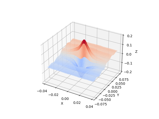
Next, we will define our test function. We are interested in generating a function that is representative of the full-field data we will use in calibrations and other MatCal studies. Generally, these data will be smooth, have some lower frequency and higher frequency behavior and may have areas of localized high gradients and values. As a result we choose, the following function which is an additive combination of three sinusoids and a linear function that is multiplied by a smooth function that approximates a dirac. This function is defined below:

def analytical_function(X,Y):
    small = H/20
    func = (H/5 * np.sin(np.pi*Y/2/(H/2)) - W/50 * X/(W/2)
           + H/40*np.sin(np.pi*Y/2/(H/20)) + W/100*np.sin(X/(W/20))) \
           * (1+small/(np.pi*(X**2+Y**2+small**2)))
    return func

We now evaluate the function on the measured grid and add noise to it with a maximum amplitude of 2.5% of the maximum value of the function on the measured grid. We then plot the function with the added noise to verify we are producing the behavior we desire.

measured_func = analytical_function(measured_x_grid, measured_y_grid)
rng = np.random.default_rng()
noise_amp = 0.025*np.max(measured_func)
noise = rng.random((measured_num_points, measured_num_points))*noise_amp-noise_amp/2
measured_func += noise

from matplotlib import cm
fig, ax = plt.subplots(subplot_kw={"projection": "3d"})
ax.plot_surface(measured_x_grid, measured_y_grid,  measured_func, cmap=cm.coolwarm)
plt.xlabel("X")
plt.ylabel("Y")
ax.set_zlabel("Z")
plt.show()

With the measured data defined, we now create the simulation grid and the truth data for the simulation grid. As stated previously, the simulation grid has 75% of the points of the measured grid and is defined on a 5% larger domain in both directions.

sim_num_points = 300
sim_xs = np.linspace(-W/2*1.025, W/2*1.025, sim_num_points)
sim_ys = np.linspace(-H/2*1.025, H/2*1.025, sim_num_points)

sim_x_grid, sim_y_grid = np.meshgrid(sim_xs, sim_ys)
sim_truth_func = analytical_function(sim_x_grid, sim_y_grid)

With the measured data and truth simulation data created, we need to prepare the data to be used with the MatCal’s interface to the Compadre GMLS tool. To do so, we convert the data to MatCal’s field data class.

measured_dict = {'x':measured_x_grid.reshape(measured_num_points**2),
                 'y':measured_y_grid.reshape(measured_num_points**2),
                 'val':measured_func.reshape(1, measured_num_points**2)}
measured_data = convert_dictionary_to_field_data(measured_dict, coordinate_names=['x','y'])

sim_truth_dict = {'x':sim_x_grid.reshape(sim_num_points**2),
                  'y':sim_y_grid.reshape(sim_num_points**2),
                  'val':sim_truth_func.reshape(1, sim_num_points**2)}
sim_truth_data = convert_dictionary_to_field_data(sim_truth_dict, coordinate_names=['x','y'])

Now we can create a set of input parameters to evaluate using our test data sets. The two input parameters to the GMLS algorithm are the local polynomial order and the search radius multiplier. Since we are going to extrapolate, we know the polynomial order should be relatively low. Also, since there is noise, we know we will want the search radius to be large enough. For the Compadre toolkit python interface, the search radius multiplier will multiply the minimum search radius needed to fit the polynomial to the region around the current point of interest. For example, a polynomial of order 1 would require 3 points for our two dimensional domain. Our interface to the Compadre toolkit, will find the two nearest neighbors to the current point of interest. The default radius will be defined as the largest distance between the current point of interest and the two other points. The search radius multiplier then scales this radius to include more points in the local polynomial fit for the current point. This is repeated for every point.

To study the influence of these parameters on our mapping tool, we perform the mapping from our measured data to our simulation grid with polynomial orders of 1 to 3 with search radius multipliers from 1.5 to 4. We than compare the mapped data to the known truth data on the simulation grid. We start by specifying the input parameters of interest and importing the GMLS tool from MatCal.

polynomial_orders =[1,2,3]
search_radius_mults = list(np.linspace(1.5,4, 11))
search_radius_mults.append(5.0)

Now we can loop over the parameters, map the measured function onto the simulation grid and calculate the error fields and error measures for the mapped field relative to the truth data on the simulation grid. We are interested in two error measures. The first error measure we will investigate is the L2-norm of the error field normalized by the maximum of the truth data on the simulation grid multiplied by 100. This is a measure of the general quality of the fit for each point on the grid it is calculated using

where is the approximated function using our GMLS mapping at the simulation grid points, is the known function evaluation at the simulation grid points and is the number of points on one axis of the grid. The second measure of error is the maximum error in the error field for all points normalized by the maximum of the truth data function and multiplied by 100. This gives a maximum percent error for the mapped data field relative to the function maximum. It is calculated using

The following code performs these calculations and stores the data in NumPy arrays so that they can be visualized next. It also stores the data in a pickle file so that it can be read back later without recalculating it since the computational cost for these mappings is expensive for the higher order polynomials and large search radius multipliers.

normalization_constant = np.max(sim_truth_func)

error_fields = []
error_norms = []
error_maxes = []
for poly_order in polynomial_orders:
    error_fields_by_search_rad = []
    error_norms_by_search_rad = []
    error_maxes_by_search_rad = []
    for search_rad_mult in search_radius_mults:
        mapped_data = meshless_remapping(measured_data, ["val"], sim_truth_data.spatial_coords,
                                         poly_order, search_rad_mult)
        error_field = mapped_data["val"]-sim_truth_data["val"]
        error_fields_by_search_rad.append(error_field)
        error_norm = np.linalg.norm(error_field)/sim_num_points**2*100/normalization_constant
        error_norms_by_search_rad.append(error_norm)
        error_max = np.max(np.abs(error_field))/normalization_constant*100
        error_maxes_by_search_rad.append(error_max)
    error_fields.append(error_fields_by_search_rad)
    error_norms.append(error_norms_by_search_rad)
    error_maxes.append(error_maxes_by_search_rad)

error_fields = np.array(error_fields)
error_norms = np.array(error_norms)
error_maxes = np.array(error_maxes)

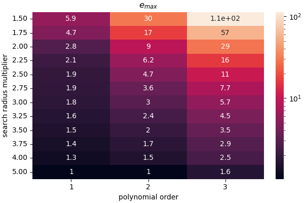
With the error fields calculated, we can now create two heat maps showing how our two error measures change as the polynomial order and search radius multiplier are varied.

from seaborn import heatmap
import matplotlib.colors as colors

search_rad_mult_labels = [f"{i:.2f}" for i in search_radius_mults]
plt.figure("$e_{{norm}}$", figsize=(6,4), constrained_layout=True)
heatmap(error_norms.T, annot=True, norm=colors.LogNorm(),
         xticklabels=polynomial_orders, yticklabels=search_rad_mult_labels)
plt.xlabel("polynomial order")
plt.ylabel("search radius multiplier")
plt.title("$e_{{norm}}$")

plt.figure("$e_{{max}}$", figsize=(6,4), constrained_layout=True)
heatmap(error_maxes.T, annot=True, norm=colors.LogNorm(),
         xticklabels=polynomial_orders, yticklabels=search_rad_mult_labels)
plt.xlabel("polynomial order")
plt.ylabel("search radius multiplier")
plt.title("$e_{{max}}$")
plt.show()

• 
• 

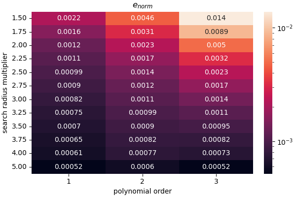
The results are somewhat expected. From the measure, we can see that linear polynomials do well at extrapolating. Since we applied a 2.5% noise centered at zero to the measured field, the best we can expect with a perfect fit is a maximum percent error on the order of 1.25%. We obtain that maximum error with linear polynomials with a search radius multiplier that is relatively large near 3.0. The other polynomial orders do not return that level of accuracy for any of the tested search radius multipliers and provide large errors when the search radius is small. From the measure, we see that overall the GMLS approximation does fairly well at reproducing the function once the search radius is large enough for all polynomials. Once again, the linear polynomial reaches the lowest values for the measure the quickest which is likely due to the extrapolation error.

We now visualize the produced error fields over the domain of interest for each set of mapping parameters used.

Note

A power norm is used for the color bar of these plot. The power norm is used to highlight the noise, but also show the maximum error. A log scale could also be used, but the level of noise was more clearly visualized with the power norm and a gamma of 0.3.

num_polys = len(polynomial_orders)
num_radiis = len(search_radius_mults)
fig= plt.figure(f"error fields for different mapping parameters",
                figsize=(5*num_polys, 5*num_radiis),
                constrained_layout=True)
max_noise_error = noise_amp/2*100/normalization_constant
for row in range(num_polys):
    for col in range(num_radiis):
        ax = plt.subplot(num_radiis, num_polys,(row+1)+num_polys*col)
        error_field = np.abs(error_fields[row, col].reshape(sim_num_points,
                                                            sim_num_points)/
                                                            normalization_constant*100)
        levs = []
        levs += list(np.linspace(0, max_noise_error, 6))
        max_err = np.max(error_field)
        if max_err > max_noise_error*3:
            levs += [max_err/2, max_err]
        elif max_err > max_noise_error:
            levs += [max_err]
        cs = ax.contourf(sim_x_grid, sim_y_grid, error_field, levs,
                         norm = colors.PowerNorm(gamma=0.3), cmap='magma')
        plt.xlabel("X")
        plt.ylabel("Y")
        plt.title(f"polynomial order {row+1}\nsearch " +
                  f"radius multiplier {search_radius_mults[col]:1.2f}")
        plt.colorbar(cs, ax=ax)
plt.show()

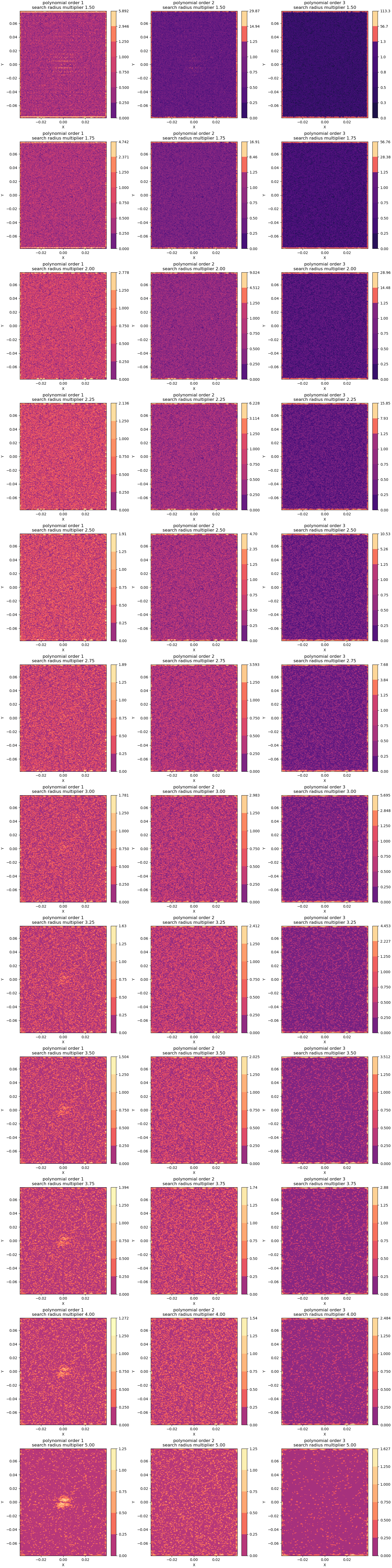
From these plots, four conclusions are clear.

1. error is highest in the extrapolation regions on the domain boundaries and the extrapolation error increases with polynomial order. As observed earlier, this is an expected result.

2. Second, the noise level seems higher in the order one polynomial. This result is expected because the high order polynomials require more neighbors and will result in a much larger window for a given search radius multiplier for this evenly spaced set of grids. By including more points, in the local least squares fit about a point more filtering of the noise is expected.

3. Third, for all polynomials orders, as the the search radius multiplier is increased the amount of filtering is also increased.

4. Fourth, the higher order polynomials perform better at the higher search radius multipliers at reproducing the smooth function of interest. For search radius multipliers greater than 3, the linear polynomial option produces noticeable error around the center where the smooth dirac function has a high amplitude.

Based on these findings, the default settings for the MatCal mapping settings are a polynomial order of 1 and a search radius multiplier of 2.75 with the goal of balancing speed and accuracy especially when extrapolation may occur.

These settings are best suited for mapping problems with the following characteristics:

1. The underlying function being studied is relatively smooth when compared to the discretization point cloud spacing. In other words, the point cloud spacing should be significantly smaller than the size of the features of interest for the function that they hold data for.

2. The data being mapped has to extrapolate a small amount away from the source data.

3. The noise in the data is small relative to the magnitude of the field of interest and only a small amount of filtering is desired.

When not extrapolating and some level of filtering is desired, the polynomial order can be increased. If extrapolating and more filtering is desired, a polynomial order of one is highly recommended, but the search radius can be increase significantly.

Note

Increasing either mapping parameter will noticeable increase run time and memory consumption.